Complete the Wikispeedia project for the Stanford CS224W course using a loop neural network
introduce
In this article, we will use modern graph machine learning techniques to conduct project practices in wikispeedia navigation paths datasets
West & Leskovec previously solved a similar problem without using graph neural networks [1]. Cordonnier & Loukas also solved this problem using a graph convolutional network of non-backtrack random walks on the Wikispeedia diagram[2]. Our technique is different from both papers and has also achieved great results.
The complete code for GitHub and Colab is also available at the end of the article.
Data + problem description
Our data comes from a collection of datasets from the Stanford Network Analysis Project (SNAP). The dataset takes navigation path data on the Wikipedia hyperlink network collected by wikipeedia players. Wikispeedia is a more puzzle mini-game called Wikiracing, where machines automatically learn common sense knowledge. The rules of the game are simple – the player chooses two different Wikipedia articles in a match, with the goal of reaching the second article with the goal of only clicking on the link provided by the first article and the sooner the better.
So what is our mission? Given that thousands of users are playing wikipedia page paths created by Wikispeedia, if we know the order of pages users have visited so far, can we predict the player's target article? Can we do this using the expressive power provided by graph neural networks?
Data preprocessing
Preparing datasets for graph machine learning requires a lot of preprocessing. The first goal is to represent the data as a directed graph with the Wikipedia article as the node and the hyperlinks that connect the articles as the edges. This step can be done using NetworkX, a Python network analysis library, and previous work by Cordonnier & Loukas [2]. Because Cordonnier & Loukas is already using Graphical Modeling Language (GML) to process and encode hyperlink graph structure files from snap datasets, we can easily import them into NetworkX.
The next goal is to process data from cordonnier & Loukas and the original SNAP dataset, which adds node-level properties to each article in the NetworkX graph. For each node, we want to include the in and out of the page and the content of the article, so here we use the average representation of the FastText pre-trained word embedding corresponding to each word in the article. Cordonnier & Loukas processed and encoded the degree of each page and the corresponding content embeddings in the text file. In addition, we categorized each article hierarchically (for example, the Cats page was classified under Science > Biology > Mammals) and added to its corresponding nodes, so Pandas was used for processing to parse tab separations and generate a multi-categorical variable for each article to indicate which categories the article belonged to. Then, by using the set_node_attributes method, the new article property is added to each corresponding node in the NetworkX graph.
import networkx as nx
# read our graph from file
our_graph = nx.read_gml('graph.gml')
# define our new node attributes
attrs = { "Cat": { "in_degree": 31 }, "New_York_City": { "in_degree": 317 } }
# add our new attributes to the graph
nx.set_node_attributes(our_graph, attrs)
The NetworkX chart is ready to load and ready to run! However, you also need to process and define the input data and labels – that is, the navigation path and the target article. Similar to the previous one, use Pandas to parse the tab-separated values of the completed navigation paths in the SNAP dataset, then process each navigation path to remove the returned click (the navigation created by the Wikipedia player returns from the current page to the previously directly visited page) and delete the last article in each path (our target article). To cleanse the data, navigation paths with more than 32 hyperlink click lengths were also removed and each navigation path was populated with 32 lengths.
This results in more than 50,000 navigation paths connected to already processed datasets of more than 4,000 different Wikipedia articles.
WikiNet model architecture
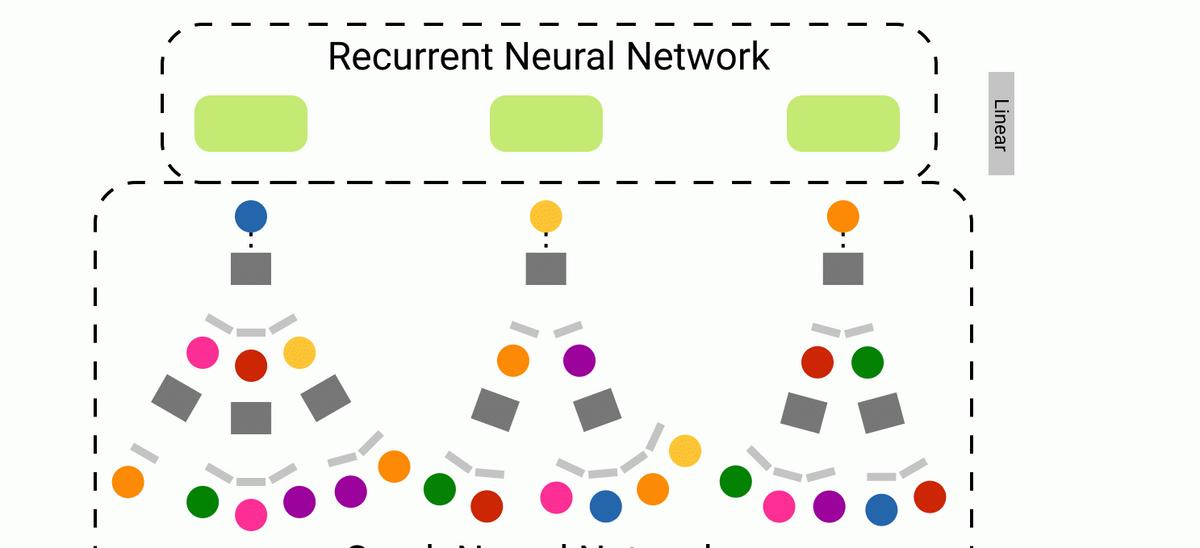
Our new approach attempts to combine the ability of recurrent neural networks (RNNs) to capture knowledge of sequences with the ability of graph neural networks (GNNs) to express graph network structures. This is The Above is WikiNet, an RNN-GNN hybrid.
import torch
import torch.nn as nn
from torch_geometric.nn import GCN # import any GNN -- we'll use GCN in this example
from torch_geometric.utils import from_networkx
# convert our networkx graph into a PyTorch Geometric (PyG) graph
pyg_graph = from_networkx(networkx_graph, group_node_attrs=NODE_ATTRIBUTE_NAMES)
# define our PyTorch model class
class Model(torch.nn.Module):
def __init__(self, pyg_graph):
super().__init__()
self.graphX = pyg_graph.x
self.graphEdgeIndex = pyg_graph.edge_index
self.gnn = GCN(in_channels=NODE_FEATURE_SIZE,
hidden_channels=GNN_HIDDEN_SIZE,
num_layers=NUM_GNN_LAYERS,
out_channels=NODE_EMBED_SIZE)
self.batch_norm_lstm = nn.BatchNorm1d(SEQUENCE_PATH_LENGTH)
self.batch_norm_linear = nn.BatchNorm1d(LSTM_HIDDEN_SIZE)
self.lstm = nn.LSTM(input_size=NODE_EMBED_SIZE,
hidden_size=LSTM_HIDDEN_SIZE,
batch_first=True)
self.pred_head = nn.Linear(LSTM_HIDDEN_SIZE, NUM_GRAPH_NODES)
def forward(self, indices):
node_emb = self.gnn(self.graphX, self.graphEdgeIndex)
node_emb_with_padding = torch.cat([node_emb, torch.zeros((1, NODE_EMBED_SIZE))])
paths = node_emb_with_padding[indices]
paths = self.batch_norm_lstm(paths)
_, (h_n, _) = self.lstm(paths)
h_n = self.batch_norm_linear(torch.squeeze(h_n))
predictions = self.pred_head(h_n)
return F.log_softmax(predictions, dim=1)
As model input, WikiNet receives a batch of page navigation paths. This is represented as a series of node indexes. Each navigation path is padded to a length of 32 — starting with a sequence of index -1 to start filling in the short sequence. The graph neural network is then used to obtain existing node properties and generate node embeddings of size 64 for each Wikipedia page in the hyperlink graph. Node embeddings that use a tensor of 0 as missing nodes (for example, those populated "nodes" denoted by index -1).
Enter this tensor into the BN layer after invoking the node embed sequence for stable training. The tensor is then fed into the RNN – in our case the LSTM model. Before the tensor is sent to the final linear layer, a BN layer is also applied to the output of the RNN. The final linear layer projects the RNN output onto one of the 4064 classes—the wiki page of the final destination. Finally, the log softmax function is applied to the output to generate probabilities.
WikiNet diagram neural network variant
There are three graph neural network styles embedded in the WikiNet experiment for generating nodes – graph convolutional networks, graph attention networks, and GraphSAGE.
First, let's discuss the general function of graph neural networks, in which the key idea is to generate node embeddings for each node based on its local neighborhood. That is, we can propagate information from its neighbors to each node.

The image above represents a calculated plot for the input plot. x_u represents the characteristics of a given node u. This is a simple example with 2 layers, although the GNN plot can be any depth. We refer to the output of node u at layer n as the "layer n embedding" of node u.
At Layer 0, the embedding of each node is given by their initial node characteristic x. At a high level, Layer K embeddings are generated from layer (k-1) embeddings by aggregating the neighbor set from each node. This inspires a two-step process for each GNN layer:
- Message calculation
- polymerization
In message computation, the k-layer embedding of the node is passed through a "message function". Use aggregate functions in aggregates to aggregate messages from node neighbors as well as the node itself. More specifically:
Graph Convolutional Neural Networks (GCN)
A simple and intuitive way to calculate messages is to use neural networks. For aggregations, you can simply take the average of the neighbor node messages. Bias terms are also used in the GCN to aggregate embeddings from the nodes themselves at the previous layer. Finally, this output is passed via an activation function such as ReLU. Thus, the equation looks like this:
Parameter matrices can be trained W_k and B_k as part of a machine learning pipeline. [3]
GraphSAGE
GraphSAGE differs from GCN in several ways. In this model, messages are computed in an aggregate function, which consists of two phases. Aggregate on the node's neighbor first — in this case, average aggregation is used. The node itself is then aggregated by embedding the previous layer of the connecting node. This connection is multiplied by a weight matrix W_k and then an activation function is used to obtain the output[4]. The overall equation embedded in the compute layer-(k+1) is as follows:
Figure Note Network (GAT)
The theoretical basis for the emergence of GAT is that not all neighbor nodes are of equal importance. GAT is similar to GCN, but instead of simply averaging aggregation, nodes are weighted using attention weights [5]. That is, the update rules are as follows:
You can see that the update rules for GCN are the same as the update rules for GAT, where:
Unlike weight matrices, note that weights are not unique to each layer. In order to calculate these attention weights, the attention coefficient is first calculated. For each node v and neighbor u, the coefficients are calculated as follows:
Then use the softmax function to calculate the final attention weight, ensuring that the sum of the weights is 1:
This allows attention weights to be trained through a weight matrix.
Training parameters
To train our model, we randomly divide our dataset into training, validation, and test datasets based on a 90/5/5% split. Use the Adam algorithm as the training optimizer, with negative log likelihood as our loss function. We used the following hyperparameters:
Experimental results
We assessed the effect of Three GNN variables of WikiNet on the prediction accuracy of the target article. This is similar to the precision@1 metric used by Cordonnier & Loukas[2]. Each GNN-RNN hybrid model has 3% to 10% higher absolute accuracy in target article predictions than pure LSTM baselines running on node features. The highest accuracy of the GNN variant using GraphSAGE as the model was 36.7%. Graph neural networks appear to have greater performance in target article predictions than the ability of graph neural networks to capture and encode local neighborhood structure information for Wikipedia pages.
cite
[1] West, R. & Leskovec, J. Human Wayfinding in Information Networks (2012), WWW 2012 — Session: Web User Behavioral Analysis and Modeling
[2] Cordonnier, J.B. & Loukas, A. Extrapolating paths with graph neural networks (2019).
[3] Kipf, T.N. & Welling, M. Semi-Supervised Classification with Graph Convolutional Networks (2017).
[4] Hamilton, W.L. & Ying, R. & Leskovec, J. Inductive Representation Learning on Large Graphs (2018).
[5] Veličković, P. et al. Graph Attention Networks (2018).
By Alexander Hurtado