excel 查询 表关联
There is a new sample file on my website, in response to a lookup question that someone asked on my Contextures Facebook page. The sample file shows how to get mileage from Excel lookup table, when you pick two cities.
我的网站上有一个新的示例文件,用于响应有人在我的Contextures Facebook页面上提出的查找问题。 该示例文件显示了当您选择两个城市时如何从Excel查询表获取里程。
Here is the question from the Facebook page:
这是Facebook页面上的问题:
I'm staring at a huge spreadsheet showing the distances in miles between a few hundred job sites…Our data is accurate, but the users often enter the wrong mileage data because it's easy to make a mistake when scrolling…
我盯着一个巨大的电子表格,该电子表格显示了数百个工作地点之间的距离(英里)……我们的数据是准确的,但是用户经常输入错误的里程数据,因为在滚动时很容易犯错误……
How can I automate this process so that I can just enter the departure site and the arrival site and retrieve the distance between the two?
如何使该过程自动化,以便我可以仅输入出发地点和到达地点并检索两者之间的距离?
里程表 (The Mileage Table)
To find data in a lookup table, based on the row and column headings, you can use the INDEX and MATCH functions. Here’s the mileage lookup table in my sample file, with cities in Florida.
要基于行和列标题在查找表中查找数据,可以使用INDEX和MATCH函数 。 这是我的示例文件中的里程查询表,其中包含佛罗里达州的城市。
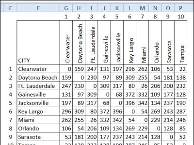
NOTE: The numbers above, and to the left of the table aren’t used – they’re just there for visual verification of the formulas.
注意:上方和表格左侧的数字未使用-它们只是用于直观验证公式的位置。
使用INDEX和MATCH (Use INDEX and MATCH)
In the sample file, data validation is used to create two drop down lists for city names, in columns A and B. In column C, an INDEX formula returns the mileage between the two selected cities.
在样本文件中,数据验证用于在A和B列中创建两个城市名称下拉列表。在C列中,INDEX公式返回两个选定城市之间的里程。
The MATCH function is used twice in the formula, to find:
在公式中两次使用了MATCH函数,以查找:
-
the row for the starting city,
起始城市所在的行,
-
the column for the destination city.
目的地城市的列。
Here’s the formula that returns the mileage:
这是返回里程的公式:
=INDEX(G3:P12, MATCH(A3,F3:F12,0), MATCH(B3,G2:P2,0))
= INDEX(G3:P12,MATCH(A3,F3:F12,0),MATCH(B3,G2:P2,0))

突出显示所选城市的里程 (Highlight the Mileage for Selected Cities)
As an extra way to verify the results, I’ve added conditional formatting in the lookup table, to highlight the cell with the mileage for the selected cities.
作为验证结果的一种额外方法,我在查找表中添加了条件格式,以突出显示带有所选城市里程的单元格。
Here is the conditional formatting formula:
这是条件格式公式:
=AND($F3=$A$3,G$2=$B$3)
= AND($ F3 = $ A $ 3,G $ 2 = $ B $ 3)
下载样本文件 (Download the Sample File)
To see the formulas and the conditional formatting, download the Get Mileage from Excel Lookup Table file from my website. On the Sample Files page, look for FN0026 – Get Travel Distance from Mileage Chart
要查看公式和条件格式,请从我的网站下载“从Excel查找表获取里程”文件。 在“示例文件”页面上,查找FN0026 –从里程表获取行进距离
The file is zipped, and in xlsx format. There are no macros in the file.
该文件已压缩,格式为xlsx。 该文件中没有宏。
观看视频 (Watch the Video)
To see the steps for creating the lookup formula, watch this short video - Get Mileage from Excel Lookup Table.
要查看创建查找公式的步骤,请观看此短片-从Excel查找表获取里程。
演示地址
翻译自: https://contexturesblog.com/archives/2013/05/09/get-mileage-from-excel-lookup-table/
excel 查询 表关联