excel 查詢 表關聯
There is a new sample file on my website, in response to a lookup question that someone asked on my Contextures Facebook page. The sample file shows how to get mileage from Excel lookup table, when you pick two cities.
我的網站上有一個新的示例檔案,用于響應有人在我的Contextures Facebook頁面上提出的查找問題。 該示例檔案顯示了當您選擇兩個城市時如何從Excel查詢表擷取裡程。
Here is the question from the Facebook page:
這是Facebook頁面上的問題:
I'm staring at a huge spreadsheet showing the distances in miles between a few hundred job sites…Our data is accurate, but the users often enter the wrong mileage data because it's easy to make a mistake when scrolling…
我盯着一個巨大的電子表格,該電子表格顯示了數百個工作地點之間的距離(英裡)……我們的資料是準确的,但是使用者經常輸入錯誤的裡程資料,因為在滾動時很容易犯錯誤……
How can I automate this process so that I can just enter the departure site and the arrival site and retrieve the distance between the two?
如何使該過程自動化,以便我可以僅輸入出發地點和到達地點并檢索兩者之間的距離?
裡程表 (The Mileage Table)
To find data in a lookup table, based on the row and column headings, you can use the INDEX and MATCH functions. Here’s the mileage lookup table in my sample file, with cities in Florida.
要基于行和列标題在查找表中查找資料,可以使用INDEX和MATCH函數 。 這是我的示例檔案中的裡程查詢表,其中包含佛羅裡達州的城市。
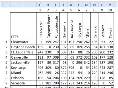
NOTE: The numbers above, and to the left of the table aren’t used – they’re just there for visual verification of the formulas.
注意:上方和表格左側的數字未使用-它們隻是用于直覺驗證公式的位置。
使用INDEX和MATCH (Use INDEX and MATCH)
In the sample file, data validation is used to create two drop down lists for city names, in columns A and B. In column C, an INDEX formula returns the mileage between the two selected cities.
在樣本檔案中,資料驗證用于在A和B列中建立兩個城市名稱下拉清單。在C列中,INDEX公式傳回兩個標明城市之間的裡程。
The MATCH function is used twice in the formula, to find:
在公式中兩次使用了MATCH函數,以查找:
-
the row for the starting city,
起始城市所在的行,
-
the column for the destination city.
目的地城市的列。
Here’s the formula that returns the mileage:
這是傳回裡程的公式:
=INDEX(G3:P12, MATCH(A3,F3:F12,0), MATCH(B3,G2:P2,0))
= INDEX(G3:P12,MATCH(A3,F3:F12,0),MATCH(B3,G2:P2,0))

突出顯示所選城市的裡程 (Highlight the Mileage for Selected Cities)
As an extra way to verify the results, I’ve added conditional formatting in the lookup table, to highlight the cell with the mileage for the selected cities.
作為驗證結果的一種額外方法,我在查找表中添加了條件格式,以突出顯示帶有所選城市裡程的單元格。
Here is the conditional formatting formula:
這是條件格式公式:
=AND($F3=$A$3,G$2=$B$3)
= AND($ F3 = $ A $ 3,G $ 2 = $ B $ 3)
下載下傳樣本檔案 (Download the Sample File)
To see the formulas and the conditional formatting, download the Get Mileage from Excel Lookup Table file from my website. On the Sample Files page, look for FN0026 – Get Travel Distance from Mileage Chart
要檢視公式和條件格式,請從我的網站下載下傳“從Excel查找表擷取裡程”檔案。 在“示例檔案”頁面上,查找FN0026 –從裡程表擷取行進距離
The file is zipped, and in xlsx format. There are no macros in the file.
該檔案已壓縮,格式為xlsx。 該檔案中沒有宏。
觀看視訊 (Watch the Video)
To see the steps for creating the lookup formula, watch this short video - Get Mileage from Excel Lookup Table.
要檢視建立查找公式的步驟,請觀看此短片-從Excel查找表擷取裡程。
示範位址
翻譯自: https://contexturesblog.com/archives/2013/05/09/get-mileage-from-excel-lookup-table/
excel 查詢 表關聯