回歸診斷主要内容
(1).誤差項是否滿足獨立性,等方差性與正态
(2).選擇線性模型是否合适
(3).是否存在異常樣本
(4).回歸分析是否對某個樣本的依賴過重,也就是模型是否具有穩定性
(5).自變量之間是否存在高度相關,是否有多重共線性現象存在
通過了t檢驗與F檢驗,但是做為回歸方程還是有問題
#舉例說明,利用anscombe資料
## 調取資料集
data(anscombe)
## 分别調取四組資料做回歸并輸出回歸系數等值
ff <- y ~ x
for(i in :) {
   ff[:] <- lapply(paste(c("y","x"), i, sep=""), as.name)
   assign(paste("lm.",i,sep=""), lmi<-lm(ff, data=anscombe))
}
GetCoef<-function(n) summary(get(n))$coef
lapply(objects(pat="lm\\.[1-4]$"), GetCoef)
[[1]]
             Estimate Std. Error  t value    Pr(>|t|)
(Intercept)
x1

[[2]]
            Estimate Std. Error  t value    Pr(>|t|)
(Intercept)
x2

[[3]]
             Estimate Std. Error  t value    Pr(>|t|)
(Intercept)
x3

[[4]]
             Estimate Std. Error  t value    Pr(>|t|)
(Intercept)
x4
從計算結果可以知道,Estimate, Std. Error,  t value,    Pr(>|t|)這幾個值完全不同,并且通過檢驗,進一步發現R^2,F值,p值完全相同,方差完全相同。事實上這四組資料完全不同,全部用線性回歸不合适。
## 繪圖
op <- par(mfrow=c(,), mar=.+c(,,,), oma=c(,,,))
for(i in :) {
    ff[2:3] <- lapply(paste(c("y","x"), i, sep=""), as.name)
    plot(ff, data =anscombe, col="red", pch=,
         bg="orange", cex=, xlim=c(,), ylim=c(,))
    abline(get(paste("lm.",i,sep="")), col="blue")
}
mtext("Anscombe's 4 Regression data sets",
       outer = TRUE, cex=)
par(op)
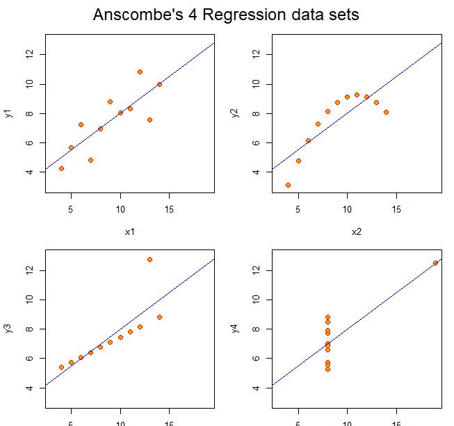
第1組資料适用于線性回歸模型,第二組使用二次模型更加合理,第三組的一個點偏離于整體資料構成的回歸直線,應該去掉。第四級做回歸是不合理的,回歸系隻依賴一個點。在得到回歸方程得到各種檢驗後,還要做相關的回歸診斷。
殘差檢驗
殘差的檢驗是檢驗模型的誤差是否滿足正态性和方差齊性,最簡單直覺的方法是畫出殘差圖。觀察殘差分布情況,作出散點圖。
#20-60歲血壓與年齡分析
## (1) 回歸
rt<-read.table("d:/R-TT/book1/1_R/chap06/blood.dat", header=TRUE)
lm.sol<-lm(Y~X, data=rt); lm.sol
summary(lm.sol)

Call:
lm(formula = Y ~ X, data = rt)

Residuals:
     Min       Q   Median       Q      Max
-  -  -

Coefficients:
            Estimate Std. Error t value Pr(>|t|)
(Intercept)         <  ***
X                     ***
---
Signif. codes:   ‘***’  ‘**’  ‘*’  ‘.’  ‘ ’

Residual standard error:  on  degrees of freedom
Multiple R-squared:  ,    Adjusted R-squared:
F-statistic:  on  and  DF,  p-value:
## (2) 殘差圖
pre<-fitted.values(lm.sol)
 #fitted value 配适值;拟合值
res<-residuals(lm.sol)
 #計算回歸模型的殘差
rst<-rstandard(lm.sol)
 #計算回歸模型标準化殘差
par(mai=c(, , , ))
plot(pre, res, xlab="Fitted Values", ylab="Residuals")
savePlot("resid-1", type="eps")

plot(pre, rst, xlab="Fitted Values",
     ylab="Standardized Residuals")
savePlot("resid-2", type="eps")

殘差
标準差
## (3) 對殘差作回歸,利用殘差絕對值與自變量(x)作回歸,其程式如下:
rt$res<-res
lm.res<-lm(abs(res)~X, data=rt); lm.res
summary(lm.res)
Call:
lm(formula = abs(res) ~ X, data = rt)

Residuals:
    Min      1Q  Median      3Q     Max
-9.7639 -2.7882 -0.1587  3.0757 10.0350

Coefficients:
            Estimate Std. Error t value Pr(>|t|)
(Intercept) -1.54948    2.18692  -0.709  0.48179
X            0.19817    0.05309   3.733  0.00047 ***
---
Signif. codes:  0 ‘***’ 0.001 ‘**’ 0.01 ‘*’ 0.05 ‘.’ 0.1 ‘ ’ 1

Residual standard error: 4.461 on 52 degrees of freedom
Multiple R-squared:  0.2113,    Adjusted R-squared:  0.1962
F-statistic: 13.93 on 1 and 52 DF,  p-value: 0.0004705
## (4) 計算殘差的标準差,利用方差(标準差的平方)的倒數作為樣本點的權重,這樣可以減少非齊性方差帶來的影響
s<-lm.res$coefficients[1]+lm.res$coefficients[2]*rt$X
lm.weg<-lm(Y~X, data=rt, weights=1/s^2); lm.weg
summary(lm.weg)
Call:
lm(formula = Y ~ X, data = rt, weights = 1/s^2)

Weighted Residuals:
    Min      1Q  Median      3Q     Max
-2.0230 -0.9939 -0.0327  0.9250  2.2008

Coefficients:
            Estimate Std. Error t value Pr(>|t|)
(Intercept) 55.56577    2.52092  22.042  < 2e-16 ***
X            0.59634    0.07924   7.526 7.19e-10 ***
---
Signif. codes:  0 ‘***’ 0.001 ‘**’ 0.01 ‘*’ 0.05 ‘.’ 0.1 ‘ ’ 1

Residual standard error: 1.213 on 52 degrees of freedom
Multiple R-squared:  0.5214,    Adjusted R-squared:  0.5122
F-statistic: 56.64 on 1 and 52 DF,  p-value: 7.187e-10