[完]機器學習實戰 第五章 Logistic回歸（Logistic Regression）

Logistic回歸的目的是尋找一個非線性函數Sigmoid的最佳拟合參數，求解過程可由最優化算法來完成，一般采用梯度上升算法，此算法又可簡化為随機梯度上升算法。簡化前後的算法效果相當，但占用更少的計算資源。并且随機梯度上升算法是一個線上算法，可在新資料到來時就完成參數的更新，而無需重新讀取整個資料集來進行批處理。機器學習的一個重要問題是處理缺失資料，處理方法取決于實際需求。

假設有一些資料點，可用一條直線對這些點進行拟合（該線稱為最佳拟合直線），這個拟合的過程就成為回歸。Logistic回歸進行分類的主要思想是：根據現有資料對分類邊界線建立回歸公式，以此進行分類。

訓練分類器用于尋找最佳拟合參數，也稱為最佳的分類回歸系數。Logistic需要距離計算，是以要求資料類型為數值型，結構化資料格式最佳。

海維賽德階躍函數（Heaviside step function）也稱為機關階躍函數，此函數的問題在于在跳躍點上從0瞬間跳躍到1，這很難處理。而Sigmoid函數，也具有類似的性質，計算公式如下：

σ(z)=11+e−z

為了實作Logistic回歸分類器，可以在每個特征上都乘以一個回歸系數，然後把所有的結果相加，将這個總和代入Sigmoid函數中，進而得到一個範圍在0~1的數值。大于0.5分入1類，否則歸入0類。

Sigmoid函數的輸入記為 z ，有下面公式得出：

z=w0x0+w1x1+w2x2+...+wnxn

采用向量寫法，上述公式可寫成 z=wTx ，其中向量 x 是分類器的輸入資料，向量w是要尋找的最佳回歸系數。

梯度上升法基于的思想：要找到某個函數的最大值，最好的方法是沿着該函數的梯度方向探尋。如果梯度記為 ∇ ，則函數 f(x,y) 的梯度由下式表示：

∇f(x,y)=⎛⎝⎜⎜⎜∂f(x,y)∂x∂f(x,y)∂y⎞⎠⎟⎟⎟

這個梯度意味着沿 x 方向移動∂f(x,y)∂x，沿 y 方向移動∂f(x,y)∂y。且函數 f(x,y) 在待計算的點上有定義且可微。

梯度算子總是指向函數值增長最快的方向。這裡說的是移動方向，而未提到移動量的大小。該量值稱為步長，記做 α 。用向量表示，梯度上升法的疊代公式如下：

w:=w+α∇wf(w)

該公式會一直疊代下去，直至達到某個停止條件為止，比如疊代次數達到某個指定值或算法達到某個可以允許的誤差範圍。

梯度上升法每次更新回歸系數時都需要周遊整個資料集，計算複雜度太高。一個改進的方法是一次僅用一個樣本點來更新回歸系數，該方法稱為随機梯度上升算法。由于可以在新樣本到來時對分類器進行增量式更新，是以，随機上升算法是一個線上學習算法，并且沒有矩陣轉換過程，所有變量的資料類型都是NumPy數組。與“線上學習”相對應，一次處理所有資料被稱為“批處理”。

随機梯度上升法，回歸系數經過大量疊代才能達到穩定值，且在大的波動停止後，仍有小的周期性波動，産生這種現象的原因是存在一些不能正确分類的樣本點（資料集并非線性可分）

改進的随機梯度上升算法，改進有兩處：1、alpha在每次疊代的時候都會調整，這可緩解資料波動或者高頻振動，雖然alpha随着疊代次數不斷減小，但永遠不會減小到0，這是因為

alpha=4/(1.0+j+i)+0.01

中存在一個常數項。這樣多次疊代之後新資料仍然具有一定的影響力。避免參數嚴格下降也常見有模拟退火算法。2、通過随機選取樣本來更新回歸系數，可減少周期性波動。

處理資料中的缺失值：1、使用可用特征的均值來填補缺失值；2、使用特殊值來填補缺失值，如-1、0，選擇使用0替換所有缺失值，恰好能适用于Logistic回歸，0在更新時不會影響系數的值；3、忽略有缺失值的樣本；4、使用相似樣本的均值填補缺失值；5、使用另外的機器學習算法預測缺失值。

如果在測試資料集中發現一條資料的類别标簽已經缺失，可簡單将其丢棄。這是因為類别标簽與特征不同，很難确定采用某個合适的值來替換。采用Logistic回歸進行分類這種做法是合理的，如果采用類似kNN的方法就可能不太可行。

使用的函數

函數	功能
mat1.transpose()	求矩陣mat1的轉置
mat(dataMat)	将輸入的資料dataMat轉換成矩陣
plt.xlabel( 'X1' )	設定x軸的文本
plt.ylabel( 'X2' )	設定y軸的文本
mat1.getA()	将mat1轉化成ndarray數組
random.uniform(x,y)	随機生成一個實數，它在[x,y]範圍内。

程式代碼

# coding=utf-8

import numpy as np

# 加載資料
def loadDataSet() :
    dataMat = []; labelMat = []
    fr = open('c:\python27\ml\\testSet.txt')
    for line in fr.readlines() :
        lineArr = line.strip().split()
        dataMat.append([, float(lineArr[]), float(lineArr[])])
        labelMat.append(int(lineArr[]))
    return dataMat, labelMat

# 階躍函數--sigmoid()函數 
def sigmoid(inX) :
    return /(+np.exp(-inX))

# logistic回歸梯度上升優化算法
def gradAscent(dataMatIn, classLabels) :
    dataMatrix = np.matrix(dataMatIn)
    labelMat = np.matrix(classLabels).transpose()
    m,n = np.shape(dataMatrix)
    # alpha項目表移動的步長
    alpha = 
    # maxCycles疊代次數
    maxCycles = 
    weights = np.ones((n,))
    for k in range(maxCycles) :
        h = sigmoid(dataMatrix*weights)
        error = labelMat - h
        # 梯度上升
        weights = weights + alpha * dataMatrix.transpose() * error
    return weights


# 畫出資料集和Logistic回歸最佳拟合直線的函數
def plotBestFit(weights) :
    import matplotlib.pyplot as plt
    dataMat, labelMat=loadDataSet()
    dataArr = np.array(dataMat)
    n = np.shape(dataArr)[]
    xcord1=[]; ycord1=[]
    xcord2=[]; ycord2=[]
    for i in range(n) :
        # 将标簽為1的資料元素和為0的分别放在(xcode1,ycode1)、(xcord2,ycord2)
        if int(labelMat[i]) ==  :
            xcord1.append(dataArr[i,])
            ycord1.append(dataArr[i,])
        else :
            xcord2.append(dataArr[i,])
            ycord2.append(dataArr[i,])
    fig = plt.figure()
    ax = fig.add_subplot()
    ax.scatter(xcord1, ycord1, s=, c='red', marker='s')
    ax.scatter(xcord2, ycord2, s=, c='green')
    # 繪制出w0 + w1*x + w2*y = 0的直線
    x = np.arange(-, , )
    y = (-weights[]-weights[]*x)/weights[]
    ax.plot(x, y)
    # x,y軸顯示的文字
    plt.xlabel('X1'); plt.ylabel('X2')
    plt.show()  

# 随機梯度上升算法
# 參數dataMatrix是numpy數組類型資料，傳入矩陣，需要np.array(matrix)轉換一下
def stocGradAscent0(dataMatrix, classLabels) :
    m,n = np.shape(dataMatrix)
    alpha = 
    weights = np.ones(n)
    # h,error 都是數值，而非向量，一次僅用一個樣本來更新回歸系數
    for i in range(m) :
        h = sigmoid(sum(dataMatrix[i]*weights))
        error = classLabels[i] - h
        weights = weights + alpha * error * dataMatrix[i]
    return weights


# 改進的随機梯度上升算法
def stocGradAscent1(dataMatrix, classLabels, numIter=) :
    m,n = np.shape(dataMatrix)
    weights = np.ones(n)
    for j in range(numIter) :
        dataIndex = range(m)
        for i in range(m) :
            # alpha每次疊代時需要調整，緩解資料波動或者高頻振動
            alpha = /(+j+i) + 
            # 随機選取更新
            randIndex = int(np.random.uniform(, len(dataIndex)))
            h = sigmoid(sum(dataMatrix[randIndex]*weights))
            error = classLabels[randIndex] - h
            weights = weights + alpha * error * dataMatrix[randIndex]
            del(dataIndex[randIndex])
    return weights

# inX, 輸入的特征向量
# weights, 回歸系數
def classifyVector(inX, weights) :
    prob = sigmoid(sum(inX*weights))
    if prob >  : return 
    else : return 

# 打開測試集和訓練集（患疝病的馬的存貨問題），使用測試集進行500疊代的Logistic回歸，
# 計算出回歸參數，并根據測試集，得出訓練模型的錯誤率
def colicTest() :
    # 打開測試集和訓練集
    frTrain = open('c:\python27\ml\\horseColicTraining.txt')
    frTest = open('c:\python27\ml\\horseColicTest.txt')
    trainingSet = []; trainingLabels = []
    for line in frTrain.readlines() :
        currLine = line.strip().split('\t')
        lineArr = []
        for i in range() :
            lineArr.append(float(currLine[i]))
        trainingSet.append(lineArr)
        trainingLabels.append(float(currLine[]))
    trainWeights = stocGradAscent1(np.array(trainingSet), trainingLabels, )
    errorCount = ; numTestVec = 
    for line in frTest.readlines() :
        numTestVec += 
        currLine = line.strip().split('\t')
        lineArr = []
        for i in range() : 
            lineArr.append(float(currLine[i]))
        if int(classifyVector(np.array(lineArr), trainWeights)) != int(currLine[]) : 
            errorCount += 
    errorRate = (float(errorCount)/numTestVec)
    print "the error rate of this test is: %f" % errorRate
    return errorRate

# 執行10次colicTest()并傳回平均值    
def multiTest() :
    numTests = ; errorSum = 
    for k in range(numTests) :
        errorSum += colicTest()
    print "after %d iterations the average error rate is: %f" \
        % (numTests, errorSum/float(numTests))      
           

在指令行中執行：

>>> import ml.logRegres as logRegres
>>> dataArr,labelMat=logRegres.loadDataSet()
>>> logRegres.gradAscent(dataArr,labelMat)
matrix([[ ],
        [ ],
        [- ]])

# 畫出資料集和決策邊界(Logistic回歸最佳拟合直線)，生成的圖，如末尾圖1
>>> import ml.logRegres as logRegres
>>> dataArr, labelMat=logRegres.loadDataSet()
>>> weights=logRegres.gradAscent(dataArr, labelMat)
>>> logRegres.plotBestFit(weights.getA())

# 随機梯度上升算法，繪制的拟合直線，如末尾圖2
>>> from numpy import *
>>> import ml.logRegres as logRegres
>>> dataArr, labelMat=logRegres.loadDataSet()
>>> weights=logRegres.stocGradAscent0(array(dataArr), labelMat)
>>> logRegres.plotBestFit(weights)

# 改進的随機梯度上升算法，繪制的拟合直線，如末尾圖3，圖4
>>> reload(logRegres)
<module 'ml.logRegres' from 'C:\Python27\ml\logRegres.py'>
>>> weights=logRegres.stocGradAscent1(array(dataArr), labelMat)
>>> logRegres.plotBestFit(weights)
>>> weights=logRegres.stocGradAscent1(array(dataArr), labelMat, )
>>> logRegres.plotBestFit(weights)

# 患有疝病的馬的存活問題
>>> reload(logRegres)
<module 'ml.logRegres' from 'C:\Python27\ml\logRegres.py'>
>>> logRegres.multiTest()
the error rate of this test is: 
the error rate of this test is: 
the error rate of this test is: 
the error rate of this test is: 
the error rate of this test is: 
the error rate of this test is: 
the error rate of this test is: 
the error rate of this test is: 
the error rate of this test is: 
the error rate of this test is: 
after  iterations the average error rate is: 
           

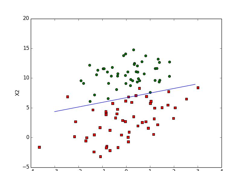
圖1 繪制資料集和決策邊界

圖2 随機梯度上升算法拟合直線

圖3 改進的随機梯度上升算法拟合直線（預設疊代150次）

圖4 改進的随機梯度上升算法拟合直線（疊代500次）