寫完畢業論文很久了,現在開始來寫這篇部落格
我的大學畢業論文是《融合圖書評論情感分析、圖書評分和使用者評分的圖書推薦系統》
其中一部分就運用到了自然語言進行中的情感分析,我用的是深度學習的方法解決,用的深度學習的Keras架構
語料資料來源于公開的ChineseNlpCorpus的資料集online_shopping_10_cats,截取其中的圖書評論資料作為後面長短記憶神經網絡的訓練集。項目位址:https://github.com/liuhuanyong/ChineseNLPCorpus
1、情感分析的語料處理
在對圖書評論的資料進行情感分析之前,去掉語料中的标點符号、特殊符号、英文字母、數字等沒用的資訊,這裡使用的是正規表達式去除,運用jieba漢語分詞庫對評論文本進行分詞。之後去掉一些停用詞,使用的是哈工大的停用詞庫,将哈工大停用詞庫的資料讀取成集合,每次對評論文本分詞後的詞語判斷是否存在于停用詞的集合當中,如果存在則去掉,否則進入下一步。最後形成一個常用詞的詞袋。
import collections
import pickle
import re
import jieba

# 資料過濾
def regex_filter(s_line):
    # 剔除英文、數字,以及空格
    special_regex = re.compile(r"[a-zA-Z0-9\s]+")
    # 剔除英文标點符号和特殊符号
    en_regex = re.compile(r"[.…{|}#$%&\'()*+,!-_./:~^;<=>?@★●,。]+")
    # 剔除中文标點符号
    zn_regex = re.compile(r"[《》、,“”;~?!:()【】]+")

    s_line = special_regex.sub(r"", s_line)
    s_line = en_regex.sub(r"", s_line)
    s_line = zn_regex.sub(r"", s_line)
    return s_line

# 加載停用詞
def stopwords_list(file_path):
    stopwords = [line.strip() for line in open(file_path, 'r', encoding='utf-8').readlines()]
    return stopwords


#主函數開始
word_freqs = collections.Counter()  # 詞頻
stopword = stopwords_list("stopWords.txt")   #加載停用詞
max_len = 0
with open("Corpus.txt", "r", encoding="utf-8",errors='ignore') as f:
    for line in f:
        comment , label = line.split(",")
        sentence = comment.replace("\n","")
        # 資料預處理
        sentence = regex_filter(sentence)   #去掉評論中的數字、字元、空格
        words = jieba.cut(sentence)   #使用jieba進行中文句子分詞
        x = 0
        for word in words:
            word_freqs[word] += 1
            x += 1                  #記錄每個詞語的詞頻
        max_len = max(max_len, x)   #将句子分詞後,記錄最長的句子長度
f.close()       #關閉檔案
with open("BookComments.txt", "r", encoding="utf-8",errors='ignore') as file:
    for line in file:
        line = line.replace("\n","")
        bookid,cm = line.split(",")
        comment_list = cm.split(";")
        for comment in comment_list:
            sentence = regex_filter(comment)   #去掉評論中的數字、字元、空格
            words = jieba.cut(sentence)   #使用jieba進行中文句子分詞
            x = 0
            for word in words:
                word_freqs[word] += 1
                x += 1                  #記錄每個詞語的詞頻
            max_len = max(max_len, x)   #将句子分詞後,記錄最長的句子長度
file.close()
print(max_len)
print('nb_words ', len(word_freqs))   #輸出詞袋的大小
2、生成字典
對語料進行處理之後,對每個詞語統計詞頻,取高頻率的詞,将每個高頻詞對應于唯一的一個數字編号,将字典寫入檔案中儲存。
## 準備資料
MAX_FEATURES = 40000 # 最大詞頻數
vocab_size = min(MAX_FEATURES, len(word_freqs)) + 2
# 建構詞頻字典
word2index = {x[0]: i+2 for i, x in enumerate(word_freqs.most_common(MAX_FEATURES))}
word2index["PAD"] = 0    #增加一個"PAD"用于後面補0的詞
word2index["UNK"] = 1    #增加一個"UNK"用于不在字典中的詞
# 将字典寫入檔案中儲存
with open('word_dict.pickle', 'wb') as handle:
    pickle.dump(word2index, handle, protocol=pickle.HIGHEST_PROTOCOL)
3、建構LSTM模型
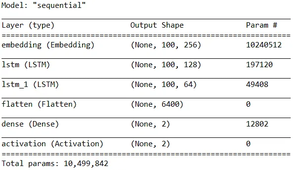
周遊資料集的每一條評論,将評論分詞,之後去掉各種無用符号和常用詞,通過上一節的字典,将詞語序列轉換成數字序列。之後劃分訓練集和測試集。先将數字序列通過Embedding嵌入層進行壓縮,轉變為詞向量[12],之後建構隐藏層大小為128和64的LSTM,通過Flatten層将資料壓平,進入Dense全連接配接層,最後進入激活層,之後構模組化型,拟合資料。其中優化器選擇adam,損失函數選擇categorical_crossentropy。
#訓練模型,找出模型的最佳疊代次數,即為4輪最佳
import pickle
from tensorflow.keras.layers import Flatten,Activation,Dense, SpatialDropout1D,Embedding,LSTM
from tensorflow.keras.models import Sequential
from tensorflow.keras.preprocessing import sequence
from sklearn.model_selection import train_test_split
from sklearn.metrics import accuracy_score, confusion_matrix, classification_report
import jieba  #用來分詞
import numpy as np
import pandas as pd
import matplotlib.pyplot as plt

# 加載分詞字典
with open('word_dict.pickle', 'rb') as handle:
    word2index = pickle.load(handle)

### 準備資料
MAX_FEATURES = 40002 # 最大詞頻數
MAX_SENTENCE_LENGTH = 100 # 句子最大長度
num_recs = 0  # 樣本數

with open("Corpus.txt", "r", encoding="utf-8",errors='ignore') as f:
    for line in f:       #周遊資料集的每一行
        num_recs += 1
f.close()

# 初始化句子數組和label數組
X = np.empty(num_recs,dtype=list)
y = np.zeros(num_recs)
i=0

with open("Corpus.txt", "r", encoding="utf-8",errors='ignore') as f:
    for line in f:
        comment , label = line.split(",")
        sentence = comment.replace(' ', '')
        words = jieba.cut(sentence)
        seqs = []
        for word in words:
            # 在詞頻中
            if word in word2index:
                seqs.append(word2index[word])
            else:
                seqs.append(word2index["UNK"]) # 不在詞頻内的補為UNK
        X[i] = seqs
        y[i] = int(label)
        i += 1
f.close()

# 把句子轉換成數字序列,并對句子進行統一長度,長的截斷,短的補0
X = sequence.pad_sequences(X, maxlen=MAX_SENTENCE_LENGTH)
# 使用pandas對label進行one-hot編碼
y1 = pd.get_dummies(y).values
print(X.shape)
print(y1.shape)
# 資料劃分
Xtrain, Xtest, ytrain, ytest = train_test_split(X, y1, test_size=0.3, random_state=0)
## 網絡建構
EMBEDDING_SIZE = 256 # 詞向量次元
HIDDEN_LAYER_SIZE = 128 # 隐藏層大小
BATCH_SIZE = 64 # 每批大小
NUM_EPOCHS = 10 # 訓練周期數


# 建立一個執行個體
model = Sequential()
# 建構詞向量
model.add(Embedding(MAX_FEATURES, EMBEDDING_SIZE,input_length=MAX_SENTENCE_LENGTH))
model.add(LSTM(HIDDEN_LAYER_SIZE, dropout=0.1, return_sequences=True))
model.add(LSTM(64, return_sequences=True))
#model.add(layers.Dropout(0.1))
model.add(Flatten())
model.add(Dense(2)) #[0, 1] or [1, 0]
model.add(Activation('softmax'))
model.compile(loss='categorical_crossentropy', optimizer='adam',metrics=['accuracy'])
model.summary()
history=model.fit(Xtrain, ytrain, epochs=10, batch_size=BATCH_SIZE, validation_data=(Xtest, ytest))
model.save('my_model.h5')
acc = history.history['accuracy']
val_acc = history.history['val_accuracy']
loss = history.history['loss']
val_loss = history.history['val_loss']

epochs = range(1, len(acc) + 1)
plt.plot(epochs, acc, 'bo', label='Training acc')
plt.plot(epochs, val_acc, 'b', label='Validation acc')
plt.title('Training and validation accuracy')
plt.legend()
plt.figure()

plt.plot(epochs, loss, 'bo', label='Training loss')
plt.plot(epochs, val_loss, 'b', label='Validation loss')
plt.title('Training and validation loss')
plt.legend()
plt.show()
LSTM的模型結構和參數
![Kafka:Topic概念與API介紹[圖]](data:image/gif;base64,R0lGODlhAQABAIAAAP///wAAACwAAAAAAQABAAACAkQBADs=)