深度学习(二)-逻辑回归

  逻辑回归很多人并不陌生，我再前面机器学习的逻辑回归：LR这一章节中也有过简单的描述。

  Logistic 回归不仅可以解决二分类问题，也可以解决多分类问题，但是二分类问题最为常见同时也具有良好的解释性 。 对于二分类问题， Logistic 回归的目标是希望找到一个区分度足够好的决策边界，能够将两类很好地分开 。而在前面我也讲过，要找到某函数的最大值，最好的方法是沿着该函数的梯度方向寻找，所以我们可以使用迭代的梯度下降来获得区分函数的最合适的参数。

  这里我使用的数据是《深度学习之pytorch》这本书中处理逻辑回归的数据，数据格式为 ( x i , y i , 类 别 ) (x_i, y_i, 类别) (xi​,yi​,类别)，首先我们获取数据，并将其可视化：

with open("./data/data.txt") as f:
	    data_list = [line.strip().split(',') for line in f.readlines()]
	    data = [(float(i[0]), float(i[1]), float(i[2])) for i in data_list]
	
	# 标准化
	x0_max = max([i[0] for i in data])
	x0_min = min([i[0] for i in data])
	x1_max = max([i[1] for i in data])
	x1_min = min([i[1] for i in data])
	data = [((i[0]-x0_min)/(x0_max-x0_min), (i[1]-x1_min)/(x1_max-x1_min), i[2]) for i in data]   # 最大最小规范化
	
	x0 = list(filter(lambda x: x[-1] == 0.0, data))  # 选择第一类的点
	x1 = list(filter(lambda x: x[-1] == 1.0, data))  # 选择第二类的点
	
	plot_x0 = [i[0] for i in x0];plot_y0 = [i[1] for i in x0]
	plot_x1 = [i[0] for i in x1];plot_y1 = [i[1] for i in x1]
	
	plt.scatter(plot_x0, plot_y0, c="r")
	plt.scatter(plot_x1, plot_y1, c="b")
	plt.show()
           

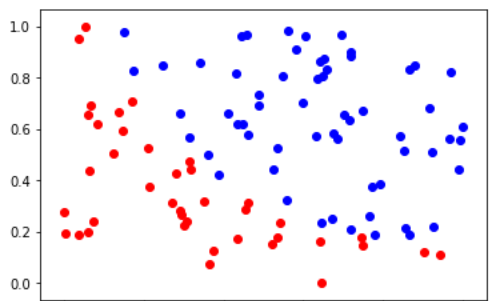
  上面的图我们可以很明显的看到数据被分为红蓝两大类，我们希望使用逻辑回归将其分开，下面开始建模型：

class LogisticRegression(nn.Module):
	    def __init__(self):
	        super(LogisticRegression, self).__init__()
	        self.lr = nn.Linear(2, 1)
	        self.sm = nn.Sigmoid()
	        
	    def forward(self, x):
	        x = self.lr(x)
	        x = self.sm(x)
	    
	        return x
	    
	model = LogisticRegression()
           

  创建损失函数与优化函数：

criterion = nn.BCEWithLogitsLoss()   # 损失函数
	optimizer = torch.optim.SGD(model.parameters(), lr=1)  # 梯度下降优化
           

  这里 n n . B C E W i t h L o g i t s L o s s nn.BCEWithLogitsLoss nn.BCEWithLogitsLoss 是二分类的损失雨数， t o r c h . o p t i m . S G D torch.optim.SGD torch.optim.SGD 是随机梯度下降优化

函数 。在训练之前我们需要讲数据转化为 V a r i a b l e Variable Variable:

np_data = np.array(data)
	x_data = torch.from_numpy(np_data[:, :-1]).float() 
	y_data = torch.from_numpy(np_data[:, -1:]).float()
	
	x_data = Variable(x_data)
	y_data = Variable(y_data)
           

  数据转换完成，开始训练：

epoch = 0
	for epoch in range(50000):
	    y_pred = model(x_data)
	
	    loss = criterion(y_pred, y_data)
	    
	    optimizer.zero_grad()   # 梯度归零
	    loss.backward()
	    optimizer.step()  # 参数更新
	
	    if epoch % 2000 == 0:
	        print('epoch {}, Loss: {:.5f}'.format((epoch), loss.data))
           

  训练完成，我们可以看到最后的模型参数 w ， b w，b w，b：

print(model.lr.weight)
	print(model.lr.bias)
           

  得到模型参数：

Parameter containing:
	tensor([[22.5674, 17.4275]], requires_grad=True)
	Parameter containing:
	tensor([-18.2705], requires_grad=True)
           

  有了模型的参数，我们可以将这条直线画出来， w w w 和 b b b 其实构成了一条直线 w 1 x + w 2 y + b = 0 w_1x + w_2y + b = 0 w1​x+w2​y+b=0 ，在直线上方是一类。

w = model.lr.weight[0]
	w0 = w.data[0].numpy()
	w1 = w.data[1].numpy()
	
	b = model.lr.bias.data[0].numpy()
	
	plot_x = np.arange(0, 1, 0.01)
	plot_y = (-w0 * plot_x - b) / w1
	
	f_y = '{:.2f}*x + {:.2f}*y + {:.2f} = 0'.format(w0, w1, b) # 打印出函数的式子
	print(f_y)
           

可以看到将两类点分开的函数为：

  画出的图形如下所示：

plt.plot(plot_x, plot_y, 'g', label='cutting line')
	plt.scatter(plot_x0, plot_y0, c="r")
	plt.scatter(plot_x1, plot_y1, c="b")