In the process of production management, the two columns of data on Saturdays and Sundays in the "Production Schedule" table are often unable to be highlighted at any time due to holidays or large and small weeks, or a lot of manpower is wasted to manually edit (the data is more energy-intensive when the data exceeds thousands of rows), resulting in the operator's pain and inefficiency.
If you are a person who is not willing to break through yourself because of repetitive work, it is definitely a good choice, the specific operation is as follows:
1. First of all, the production schedule we get is shown in the following figure (in fact, the one you use and our case will be very different, but it is not important, the operation method is the same)
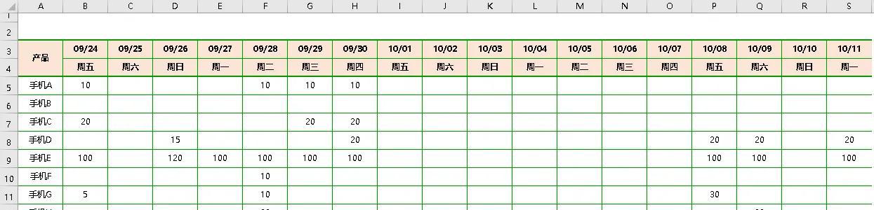
Just an example!!!
Because facing the 11th National Day holiday, September began to arrange a holiday, but as C column (9/25th) Saturday did not go to work, no scheduled production, but could not understand the first time, the visualization effect is not good ~
Of course, we can add the upper color to the area by selecting the C5:C13, I5:O13, R5:R13 range, by selecting the color, as shown in the following figure

It can be manipulated when the planning span is small or when there is little data, but it is not conducive to sustainable use
But this also has a problem, this case only has 14 rows, the actual application process data will be much greater than the secondary data (more than 1000 rows, 5000 rows, etc.), dragging down when selecting may have made you give up, and you have to choose countless times, every weekend to choose
2. Mouse drag to select the A5:R13 range (you want to increase the formatting of the area, you can also Ctrl+A (Select All)), select Conditional Formatting – New Rule
3. Select "Use formula to determine which cells to format", and enter =A$2="Rest Day" in the rule, click OK
note:
- Use A2 cell to set the rule, please note that the selected range is A5:R13, the "represented cell" used in the setting formula must be the first row of the selection range or a cell of the first column
- A$2 is the whole column to increase color, $A 2 is to add color to the entire row
4. The final effect after entering "Rest Day" in row 2 of the table is as follows
You only need to select the area once when setting the conditional formatting, and adjust the cell where the "rest day" is located, the rest day content entry can be combined with the drop-down menu or use the IF formula to automatically enter the cell content = rest day when the 3rd row is Saturday or Sunday, if this is not good, you can change the rest day to other symbols, of course, the conditional formatting must also be modified simultaneously!
There are many methods, and we look forward to developing them together!
Personally feel that this method is relatively simple, the burden of program operation is also small, other methods are also available, but a little complicated, if you have a good method, welcome to leave a message to communicate, learning is learned in continuous practice, look forward to everyone to communicate together.