Convolutional Neural Networks
使用全連接配接層的局限性:
- 圖像在同一列鄰近的像素在這個向量中可能相距較遠。它們構成的模式可能難以被模型識别。
- 對于大尺寸的輸入圖像,使用全連接配接層容易導緻模型過大。
使用卷積層的優勢:
- 卷積層保留輸入形狀。
- 卷積層通過滑動視窗将同一卷積核與不同位置的輸入重複計算,進而避免參數尺寸過大。
LeNet 模型
LeNet分為卷積層塊和全連接配接層塊兩個部分。下面我們分别介紹這兩個子產品。
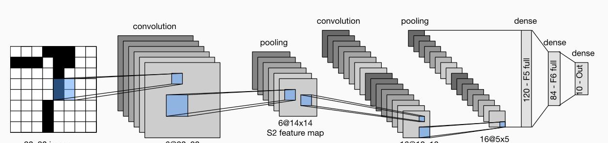
卷積層塊裡的基本機關是卷積層後接平均池化層:卷積層用來識别圖像裡的空間模式,如線條和物體局部,之後的平均池化層則用來降低卷積層對位置的敏感性。
卷積層塊由兩個這樣的基本機關重複堆疊構成。在卷積層塊中,每個卷積層都使用 5 × 5 5 \times 5 5×5的視窗,并在輸出上使用sigmoid激活函數。第一個卷積層輸出通道數為6,第二個卷積層輸出通道數則增加到16。
全連接配接層塊含3個全連接配接層。它們的輸出個數分别是120、84和10,其中10為輸出的類别個數。
下面我們通過Sequential類來實作LeNet模型。
#import
import sys
sys.path.append("/home/kesci/input")
import d2lzh1981 as d2l
import torch
import torch.nn as nn
import torch.optim as optim
import time
#net
class Flatten(torch.nn.Module):  #展平操作
    def forward(self, x):
        return x.view(x.shape[0], -1)

class Reshape(torch.nn.Module): #将圖像大小重定型
    def forward(self, x):
        return x.view(-1,1,28,28)      #(B x C x H x W)

net = torch.nn.Sequential(     #Lelet
    Reshape(),
    nn.Conv2d(in_channels=1, out_channels=6, kernel_size=5, padding=2), #b*1*28*28  =>b*6*28*28
    nn.Sigmoid(),
    nn.AvgPool2d(kernel_size=2, stride=2),                              #b*6*28*28  =>b*6*14*14
    nn.Conv2d(in_channels=6, out_channels=16, kernel_size=5),           #b*6*14*14  =>b*16*10*10
    nn.Sigmoid(),
    nn.AvgPool2d(kernel_size=2, stride=2),                              #b*16*10*10  => b*16*5*5
    Flatten(),                                                          #b*16*5*5   => b*400
    nn.Linear(in_features=16*5*5, out_features=120),
    nn.Sigmoid(),
    nn.Linear(120, 84),
    nn.Sigmoid(),
    nn.Linear(84, 10)
)
接下來我們構造一個高和寬均為28的單通道資料樣本,并逐層進行前向計算來檢視每個層的輸出形狀。
#print
X = torch.randn(size=(1,1,28,28), dtype = torch.float32)
for layer in net:
    X = layer(X)
    print(layer.__class__.__name__,'output shape: \t',X.shape)
Reshape output shape: 	 torch.Size([1, 1, 28, 28])
Conv2d output shape: 	 torch.Size([1, 6, 28, 28])
Sigmoid output shape: 	 torch.Size([1, 6, 28, 28])
AvgPool2d output shape: 	 torch.Size([1, 6, 14, 14])
Conv2d output shape: 	 torch.Size([1, 16, 10, 10])
Sigmoid output shape: 	 torch.Size([1, 16, 10, 10])
AvgPool2d output shape: 	 torch.Size([1, 16, 5, 5])
Flatten output shape: 	 torch.Size([1, 400])
Linear output shape: 	 torch.Size([1, 120])
Sigmoid output shape: 	 torch.Size([1, 120])
Linear output shape: 	 torch.Size([1, 84])
Sigmoid output shape: 	 torch.Size([1, 84])
Linear output shape: 	 torch.Size([1, 10])
可以看到,在卷積層塊中輸入的高和寬在逐層減小。卷積層由于使用高和寬均為5的卷積核,進而将高和寬分别減小4,而池化層則将高和寬減半,但通道數則從1增加到16。全連接配接層則逐層減少輸出個數,直到變成圖像的類别數10。

擷取資料和訓練模型
下面我們來實作LeNet模型。我們仍然使用Fashion-MNIST作為訓練資料集。
# 資料
batch_size = 256
train_iter, test_iter = d2l.load_data_fashion_mnist(
    batch_size=batch_size, root='/home/kesci/input/FashionMNIST2065')
print(len(train_iter))
235
為了使讀者更加形象的看到資料,添加額外的部分來展示資料的圖像
#資料展示
import matplotlib.pyplot as plt
def show_fashion_mnist(images, labels):
    d2l.use_svg_display()
    # 這裡的_表示我們忽略(不使用)的變量
    _, figs = plt.subplots(1, len(images), figsize=(12, 12))
    for f, img, lbl in zip(figs, images, labels):
        f.imshow(img.view((28, 28)).numpy())
        f.set_title(lbl)
        f.axes.get_xaxis().set_visible(False)
        f.axes.get_yaxis().set_visible(False)
    plt.show()

for Xdata,ylabel in train_iter:
    break
X, y = [], []
for i in range(10):
    print(Xdata[i].shape,ylabel[i].numpy())
    X.append(Xdata[i]) # 将第i個feature加到X中
    y.append(ylabel[i].numpy()) # 将第i個label加到y中
show_fashion_mnist(X, y)
torch.Size([1, 28, 28]) 3
torch.Size([1, 28, 28]) 8
torch.Size([1, 28, 28]) 1
torch.Size([1, 28, 28]) 4
torch.Size([1, 28, 28]) 0
torch.Size([1, 28, 28]) 0
torch.Size([1, 28, 28]) 4
torch.Size([1, 28, 28]) 9
torch.Size([1, 28, 28]) 4
torch.Size([1, 28, 28]) 7
因為卷積神經網絡計算比多層感覺機要複雜,建議使用GPU來加速計算。我們檢視看是否可以用GPU,如果成功則使用
cuda:0
,否則仍然使用
cpu
。
# This function has been saved in the d2l package for future use
#use GPU
def try_gpu():
    """If GPU is available, return torch.device as cuda:0; else return torch.device as cpu."""
    if torch.cuda.is_available():
        device = torch.device('cuda:0')
    else:
        device = torch.device('cpu')
    return device

device = try_gpu()
device
device(type='cpu')
我們實作
evaluate_accuracy
函數,該函數用于計算模型
net
在資料集
data_iter
上的準确率。
#計算準确率
'''
(1). net.train()
  啟用 BatchNormalization 和 Dropout,将BatchNormalization和Dropout置為True
(2). net.eval()
不啟用 BatchNormalization 和 Dropout,将BatchNormalization和Dropout置為False
'''

def evaluate_accuracy(data_iter, net,device=torch.device('cpu')):
    """Evaluate accuracy of a model on the given data set."""
    acc_sum,n = torch.tensor([0],dtype=torch.float32,device=device),0
    for X,y in data_iter:
        # If device is the GPU, copy the data to the GPU.
        X,y = X.to(device),y.to(device)
        net.eval()
        with torch.no_grad():
            y = y.long()
            acc_sum += torch.sum((torch.argmax(net(X), dim=1) == y))  #[[0.2 ,0.4 ,0.5 ,0.6 ,0.8] ,[ 0.1,0.2 ,0.4 ,0.3 ,0.1]] => [ 4 , 2 ]
            n += y.shape[0]
    return acc_sum.item()/n
我們定義函數
train_ch5
,用于訓練模型。
#訓練函數
def train_ch5(net, train_iter, test_iter,criterion, num_epochs, batch_size, device,lr=None):
    """Train and evaluate a model with CPU or GPU."""
    print('training on', device)
    net.to(device)
    optimizer = optim.SGD(net.parameters(), lr=lr)
    for epoch in range(num_epochs):
        train_l_sum = torch.tensor([0.0],dtype=torch.float32,device=device)
        train_acc_sum = torch.tensor([0.0],dtype=torch.float32,device=device)
        n, start = 0, time.time()
        for X, y in train_iter:
            net.train()

            optimizer.zero_grad()
            X,y = X.to(device),y.to(device)
            y_hat = net(X)
            loss = criterion(y_hat, y)
            loss.backward()
            optimizer.step()

            with torch.no_grad():
                y = y.long()
                train_l_sum += loss.float()
                train_acc_sum += (torch.sum((torch.argmax(y_hat, dim=1) == y))).float()
                n += y.shape[0]
        test_acc = evaluate_accuracy(test_iter, net,device)
        print('epoch %d, loss %.4f, train acc %.3f, test acc %.3f, '
              'time %.1f sec'
              % (epoch + 1, train_l_sum/n, train_acc_sum/n, test_acc,
                 time.time() - start))
我們重新将模型參數初始化到對應的裝置
device
(
cpu
or
cuda:0
)之上,并使用Xavier随機初始化。損失函數和訓練算法則依然使用交叉熵損失函數和小批量随機梯度下降。
# 訓練
lr, num_epochs = 0.9, 10

def init_weights(m):
    if type(m) == nn.Linear or type(m) == nn.Conv2d:
        torch.nn.init.xavier_uniform_(m.weight)

net.apply(init_weights)
net = net.to(device)

criterion = nn.CrossEntropyLoss()   #交叉熵描述了兩個機率分布之間的距離,交叉熵越小說明兩者之間越接近
train_ch5(net, train_iter, test_iter, criterion,num_epochs, batch_size,device, lr)
training on cpu
epoch 1, loss 0.0091, train acc 0.100, test acc 0.168, time 21.6 sec
epoch 2, loss 0.0065, train acc 0.355, test acc 0.599, time 21.5 sec
epoch 3, loss 0.0035, train acc 0.651, test acc 0.665, time 21.8 sec
epoch 4, loss 0.0028, train acc 0.717, test acc 0.723, time 21.7 sec
epoch 5, loss 0.0025, train acc 0.746, test acc 0.753, time 21.4 sec
epoch 6, loss 0.0023, train acc 0.767, test acc 0.754, time 21.5 sec
epoch 7, loss 0.0022, train acc 0.782, test acc 0.785, time 21.3 sec
epoch 8, loss 0.0021, train acc 0.798, test acc 0.791, time 21.8 sec
epoch 9, loss 0.0019, train acc 0.811, test acc 0.790, time 22.0 sec
epoch 10, loss 0.0019, train acc 0.821, test acc 0.804, time 22.1 sec
# test
for testdata,testlabe in test_iter:
    testdata,testlabe = testdata.to(device),testlabe.to(device)
    break
print(testdata.shape,testlabe.shape)
net.eval()
y_pre = net(testdata)
print(torch.argmax(y_pre,dim=1)[:10])
print(testlabe[:10])
torch.Size([256, 1, 28, 28]) torch.Size([256])
tensor([9, 2, 1, 1, 6, 1, 2, 6, 5, 7])
tensor([9, 2, 1, 1, 6, 1, 4, 6, 5, 7])
總結:
卷積神經網絡就是含卷積層的網絡。
LeNet交替使用卷積層和最大池化層後接全連接配接層來進行圖像分類。
net.eval()
y_pre = net(testdata)
print(torch.argmax(y_pre,dim=1)[:10])
print(testlabe[:10])
torch.Size([256, 1, 28, 28]) torch.Size([256])
    tensor([9, 2, 1, 1, 6, 1, 2, 6, 5, 7])
    tensor([9, 2, 1, 1, 6, 1, 4, 6, 5, 7])


## 總結:

卷積神經網絡就是含卷積層的網絡。
LeNet交替使用卷積層和最大池化層後接全連接配接層來進行圖像分類。