✅作者簡介:熱愛科研的Matlab仿真開發者,修心和技術同步精進。
🍎個人首頁:Matlab科研工作室
🍊個人信條:格物緻知。
更多Matlab仿真内容點選👇
智能優化算法 神經網絡預測 雷達通信 無線傳感器
信号處理 圖像處理 路徑規劃 元胞自動機 無人機
⛄ 内容介紹
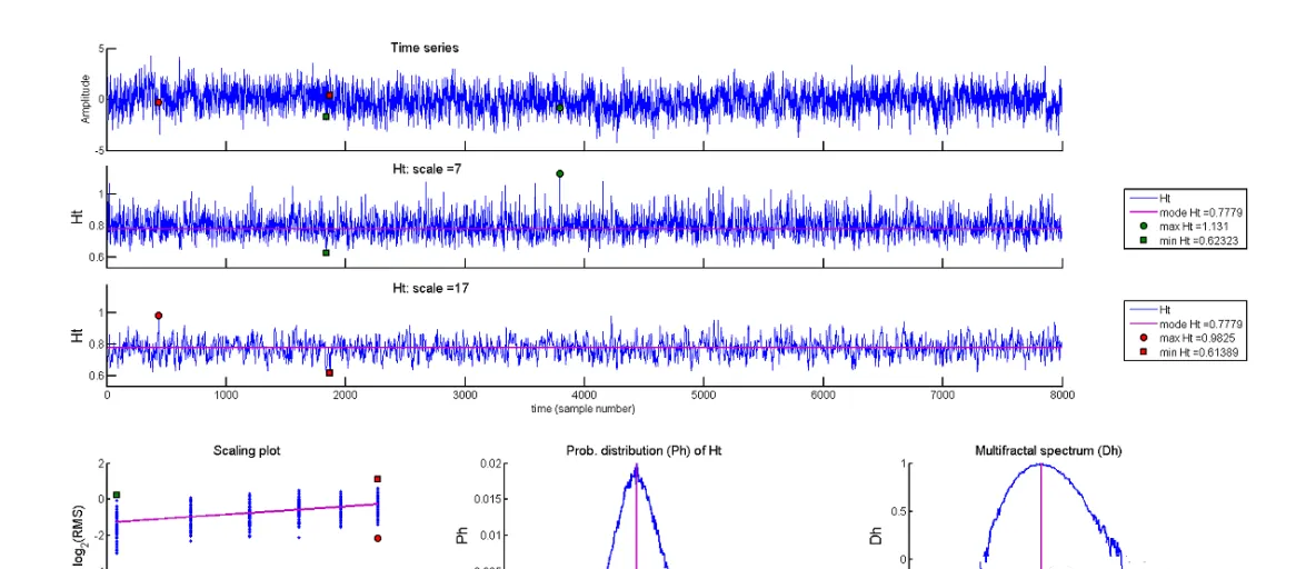
Fractal structures are found in biomedical time series from a wide range of physiological
phenomena. The multifractal spectrum identififies the deviations in fractal structure within
time periods with large and small flfluctuations. The present tutorial is an introduction to
multifractal detrended flfluctuation analysis (MFDFA) that estimates the multifractal spec
trum of biomedical time series. The tutorial presents MFDFA step-by-step in an interactive
Matlab session. All Matlab tools needed are available in Introduction to MFDFA folder at the
website www.ntnu.edu/inm/geri/software. MFDFA are introduced in Matlab code boxes
where the reader can employ pieces of, or the entire MFDFA to example time series. After
introducing MFDFA, the tutorial discusses the best practice of MFDFA in biomedical signal
processing. The main aim of the tutorial is to give the reader a simple self-sustained guide
to the implementation of MFDFA and interpretation of the resulting multifractal spectra.
⛄ 部分代碼
YMatrix1=[multifractal.*30,RW3];
YMatrix2=[monofractal.*30,RW2];
YMatrix3=[whitenoise.*30,RW1];
X1=2600:3600;
Y1=RW3(2600:3600);
% Create figure
figure1 = figure('PaperType','a4letter','PaperSize',[20.98 29.68],...
'Color',[1 1 1]);
% Create axes
axes1 = axes('Parent',figure1,'YTickLabel',{'0','200','400','600'},...
'YTick',[0 200 400 600],...
'XTickLabel',{},...
'XTick',zeros(1,0),...
'Position',[0.13 0.6545 0.7745 0.2705],...
'LineWidth',2,...
'FontSize',14);
% Uncomment the following line to preserve the Y-limits of the axes
ylim(axes1,[-220 700]);
hold(axes1,'all');
% Create multiple lines using matrix input to plot
pplot1 = plot(YMatrix1,'Parent',axes1);
set(pplot1(2),'LineWidth',2,'Color',[1 0 0]);
% Create axes
axes2 = axes('Parent',figure1,'YTickLabel',{},'YTick',zeros(1,0),...
'XTick',zeros(1,0),...
'Position',[0.6641 0.8264 0.1875 0.1359],...
'LineWidth',2);
% Uncomment the following line to preserve the Y-limits of the axes
ylim(axes2,[370 570]);
box(axes2,'on');
hold(axes2,'all');
% Create plot
plot(X1,Y1,'Parent',axes2,'LineWidth',2,'Color',[1 0 0]);
% Create axes
axes3 = axes('Parent',figure1,'YTickLabel',{'0','200','400','600'},...
'YTick',[0 200 400 600],...
'XTickLabel',{},...
'XTick',zeros(1,0),...
'Position',[0.13 0.3833 0.7745 0.272],...
'LineWidth',2,...
'FontSize',14);
% Uncomment the following line to preserve the Y-limits of the axes
ylim(axes3,[-220 700]);
hold(axes3,'all');
% Create multiple lines using matrix input to plot
pplot2 = plot(YMatrix2,'Parent',axes3);
set(pplot2(1),'DisplayName','Noise like time series');
set(pplot2(2),'LineWidth',2,'Color',[1 0 0],...
'DisplayName','Random walk like time series');
% Create ylabel
ylabel('Amplitude (measurement units)','FontSize',14);
% Create axes
axes4 = axes('Parent',figure1,'YTickLabel',{'-200','0','200','400','600'},...
'YTick',[0 200 400 600],...
'XTickLabel',{'0','1?00','2?00','3?00','4?00','5?00','6?00','7?00','8?00'},...
'XTick',[0 1000 2000 3000 4000 5000 6000 7000 8000],...
'Position',[0.13 0.1108 0.7745 0.2723],...
'LineWidth',2,...
'FontSize',14);
ylim(axes4,[-220 700]);
hold(axes4,'all');
% Create multiple lines using matrix input to plot
pplot3 = plot(YMatrix3,'Parent',axes4);
set(pplot3(2),'LineWidth',2,'Color',[1 0 0]);
% Create xlabel
xlabel('time (sample number)','FontSize',14);
% Create legend
legend1 = legend(axes3,'show');
set(legend1,'LineWidth',2);
% Create textbox
annotation(figure1,'textbox',[0.2362 0.6476 0.1934 0.04038],...
'String',{'Monofractal time series'},...
'FontSize',14,...
'FitBoxToText','off',...
'LineStyle','none');
% Create textbox
annotation(figure1,'textbox',[0.2362 0.9246 0.1822 0.04038],...
'String',{'Multifractal time series'},...
'FontSize',14,...
'FitBoxToText','off',...
'LineStyle','none');
% Create textbox
annotation(figure1,'textbox',[0.238 0.2453 0.1057 0.04038],...
'String',{'White noise'},...
'FontSize',14,...
'FitBoxToText','off',...
'LineStyle','none');
% Create line
annotation(figure1,'line',[0.3828 0.3828],[0.8978 0.8278]);
% Create line
annotation(figure1,'line',[0.3828 0.4714],[0.8281 0.8291]);
% Create line
annotation(figure1,'line',[0.4713 0.4713],[0.8294 0.9004]);
% Create line
annotation(figure1,'line',[0.3828 0.4705],[0.8995 0.9004]);
% Create line
annotation(figure1,'line',[0.4705 0.6632],[0.8291 0.8277]);
% Create line
annotation(figure1,'line',[0.4696 0.6667],[0.9017 0.9637]);
% Create line
annotation(figure1,'line',[0.1302 0.1293],[0.9327 0.8977],'LineWidth',4,...
'Color',[1 1 1]);
clear pplot1 pplot2 pplot3 legend1 axes1 figure1 axes2 figure2 axes3 figure3 ans axes4 X1 Y1 YMatrix1 YMatrix2 YMatrix3
⛄ 運作結果

編輯
編輯
編輯
編輯
編輯
編輯
編輯
正在上傳…重新上傳取消
編輯
編輯
編輯
⛄ 參考文獻
[1]Espen Alexander Fürst E.A.F.I. Ihlen. Introduction to Multifractal Detrended Fluctuation Analysis in Matlab[J]. Frontiers, 2012.