時間序列基于監督學習的LSTM模型為什麼可以預測股票走勢（附完整代碼）

疫情期間，在家學習Python，調通了基于監督學習的LSTM神經網絡預測模型代碼，在一般代碼的基礎上，做了單步和多步通用版的改進。調通的代碼附後，供各位大咖指正。

雖然代碼調通了，但是發現輸出的預測結果均滞後于實際值，更像是對原始資料的拟合而不是預測，這個文章主要是想請教一下：

1、代碼問題在哪裡？

2、如果代碼沒問題，預測功能是怎麼展現的？

3、如果有類似的群，友善也請大咖告知，可以加群學習，謝謝。

import pandas as pd 
# 設定顯示的最大列、寬等參數，消掉列印不完全中間的省略号
pd.set_option('display.max_columns', 1000)
pd.set_option('display.width', 1000)
pd.set_option('display.max_colwidth', 1000)
import matplotlib.pyplot as plt
import tensorflow as tf
import os
from pandas import read_excel
import numpy as np
from pandas import DataFrame
from pandas import concat
from sklearn.preprocessing import MinMaxScaler
from keras.models import Sequential, load_model
from keras.layers import LSTM, Dense, Dropout, BatchNormalization
from numpy import concatenate
from sklearn.metrics import mean_squared_error, mean_absolute_error, r2_score
from math import sqrt

# 定義參數
start_rate = 0.99
end_rate = 0.01
n_features = 21  # 特征值數
n_predictions = 1  # 預測值數
delay = 5  # 目标是未來第5個交易日
test_trade_date = []


# 定義字元串轉換為浮點型
def str_to_float(s):
    s = s[:-1]
    s_float = float(s)
    return s_float


# 定義series_to_supervised()函數
# 将時間序列轉換為監督學習問題
def series_to_supervised(data, n_in=1, n_out=1, dropnan=True):
    """
    Frame a time series as a supervised learning dataset.
    Arguments:
        data: Sequence of observations as a list or NumPy array.
        n_in: Number of lag observations as input (X).
        n_out: Number of observations as output (y).
        dropnan: Boolean whether or not to drop rows with NaN values.
    Returns:
        Pandas DataFrame of series framed for supervised learning.
    """
    n_vars = 1 if type(data) is list else data.shape[1]
    df = DataFrame(data)
    cols, names = list(), list()
    # input sequence (t-n, ... t-1)輸入序列
    for i in range(n_in, 0, -1):
        cols.append(df.shift(i))
        names += [('var%d(t-%d)' % (j + 1, i)) for j in range(n_vars)]
    # forecast sequence (t, t+1, ... t+n)預測序列
    for i in range(0, n_out):
        cols.append(df.shift(-i))
        if i == 0:
            names += [('var%d(t)' % (j + 1)) for j in range(n_vars)]
        else:
            names += [('var%d(t+%d)' % (j + 1, i)) for j in range(n_vars)]
    # put it all together
    agg = concat(cols, axis=1)
    agg.columns = names
    # drop rows with NaN values
    nan_rows = agg[agg.isnull().T.any().T]
    if dropnan:
        agg.dropna(inplace=True)
    return agg


def generator(tsc='000001', delay=5):
    # 讀取檔案，删除不必要項
    stock_data = pd.read_csv(r"c:\python\日k線資料\%s.csv" % tsc, index_col=0)  # 讀入股票資料,防止第一列被當作資料，加入index_col=0
    stock_data['schange'] = stock_data['close']
    stock_data.reset_index(drop=True, inplace=True)
    stock_data.drop(['ts_code', 'trade_date', 'pre_close', 'change', 'pct_chg'], axis=1,
                    inplace=True)  # df=df.iloc[:,1:13]
    # 缺失值填充
    stock_data.fillna(method='bfill', inplace=True)
    stock_data.fillna(method='ffill', inplace=True)
    # 列印資料的後5行
    n_features = len(stock_data.columns)
    # 擷取DataFrame中的資料，形式為數組array形式
    values = stock_data.values
    # 確定所有資料為float類型
    values = values.astype('float32')
    # 特征的歸一化處理
    scaler = MinMaxScaler(feature_range=(0, 1))
    # 資料一起處理再分訓練集、測試集
    scaled = scaler.fit_transform(values)
    row = len(scaled)
    reframed = series_to_supervised(scaled, delay, 1)
    # 把資料分為訓練集和測試集
    values = reframed.values
    train_end = int(np.floor(start_rate * row))
    test_start = train_end
    train = values[:train_end, :]
    test = values[test_start:, :]
    # 把資料分為輸入和輸出
    n_obs = delay * n_features
    # 分離特征集和标簽
    train_X, train_y = train[:, :n_obs], train[:, -n_predictions]
    test_X, test_y = test[:, :n_obs], test[:, -n_predictions]

    # 把輸入重塑成3D格式 [樣例， 時間步, 特征]
    train_X = train_X.reshape((train_X.shape[0], 1, train_X.shape[1]))
    test_X = test_X.reshape((test_X.shape[0], 1, test_X.shape[1]))
    # 轉化為三維資料,reshape input to be 3D [samples, timesteps, features]
    train_X = train_X.reshape((train_X.shape[0], delay, n_features))
    test_X = test_X.reshape((test_X.shape[0], delay, n_features))
    return train_X, train_y, test_X, test_y, scaler


# 搭建LSTM模型
train_X, train_y, test_X, test_y, scaler = generator()
model = Sequential()
model.add(LSTM(20, input_shape=(train_X.shape[1], train_X.shape[2]), return_sequences=True))
model.add(LSTM(units=20))
model.add(Dropout(0.5))
model.add(Dense(1, activation='relu'))
model.compile(loss='mean_squared_error', optimizer='adam')  # fit network  'mean_squared_error''mae'
history = model.fit(train_X, train_y, epochs=500, batch_size=100, validation_data=(test_X, test_y), verbose=2,
                    shuffle=False)
model.save('c:\python\model\model')
# 繪制損失圖
plt.plot(history.history['loss'], label='train')
plt.plot(history.history['val_loss'], label='test')
plt.title('LSTM_000001.SZ', fontsize='12')
plt.ylabel('loss', fontsize='10')
plt.xlabel('epoch', fontsize='10')
plt.legend()
plt.show()

print("訓練完成，開始預測……")
model = tf.keras.models.load_model('c:\python\model\model')
# 模型預測收益率
y_predict = model.predict(test_X)
n_features = test_X.shape[2]
# model.save(SAVE_PATH + 'model')
test_X = test_X.reshape((test_X.shape[0], test_X.shape[1] * test_X.shape[2]))

# 将預測結果按比例反歸一化
inv_y_test = concatenate((test_X[:, -n_features:-1], y_predict), axis=1)
inv_y_test = scaler.inverse_transform(inv_y_test)
inv_y_predict = inv_y_test[:, -1]

# invert scaling for actual
# #将真實結果按比例反歸一化
test_y = test_y.reshape((len(test_y), 1))
inv_y_train = concatenate((test_X[:, -n_features:-1], test_y), axis=1)
inv_y_train = scaler.inverse_transform(inv_y_train)
inv_y = inv_y_train[:, -1]
print('反歸一化後的預測結果：', inv_y_predict)
print('反歸一化後的真實結果：', inv_y)

# 寫入檔案
df = pd.DataFrame()
df['e'] = inv_y
df['pe'] = inv_y_predict
df.to_csv("c:\python\predict_result.csv")
# 繪圖
'''
inv_y=inv_y[delay:,]
#inv_y=inv_y[:-delay,]
for i in range(delay):
    #inv_y=np.concatenate((inv_y,inv_y[-1:,]) , axis=0)
    inv_y = np.concatenate((inv_y[0:1, ],inv_y), axis=0)
'''
plt.plot(inv_y, color='red', label='Original')
plt.plot(inv_y_predict, color='green', label='Predict')
plt.xlabel('the number of test data')
plt.ylabel('5dayearn')
plt.title('predict')
plt.legend()
plt.show()

# 回歸評價名額
# calculate MSE 均方誤差
mse = mean_squared_error(inv_y, inv_y_predict)
# calculate RMSE 均方根誤差
rmse = sqrt(mean_squared_error(inv_y, inv_y_predict))
# calculate MAE 平均絕對誤差
mae = mean_absolute_error(inv_y, inv_y_predict)
# calculate R square
r_square = r2_score(inv_y, inv_y_predict)
print('均方誤差(mse): %.6f' % mse)
print('均方根誤差(rmse): %.6f' % rmse)
print('平均絕對誤差(mae): %.6f' % mae)
print('R_square: %.6f' % r_square)           

複制

用代碼生成5日資料預測和實際值對比圖如下圖所示：

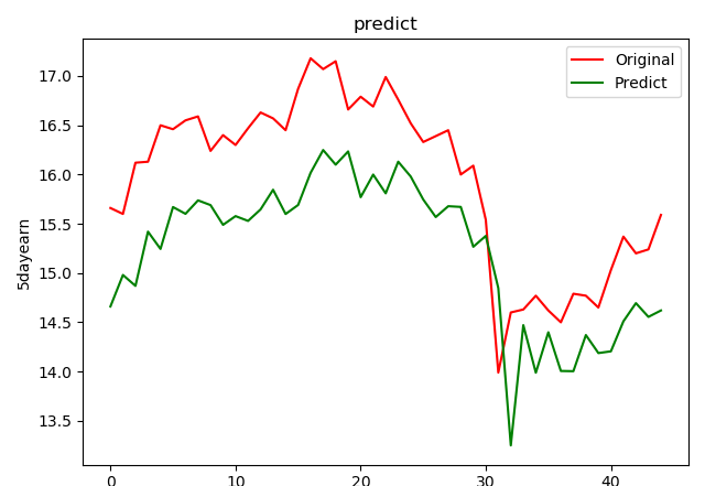
5日資料預測值和真實值對比圖

預測品質評價資料如下：

均方誤差(mse): 0.673632

均方根誤差(rmse): 0.820751

平均絕對誤差(mae): 0.770078

R_square: 0.067422

調試時發現，如果在開始階段将訓練集和測試集分别進行歸一化處理，預測資料品質更好，

圖像的拟合程度更高，同樣也能更明顯的看出預測資料的滞後性：

在開始階段将訓練集和測試集分别進行歸一化處理

預測品質評價資料如下：

均方誤差(mse): 0.149244

均方根誤差(rmse): 0.386321

平均絕對誤差(mae): 0.285039

R_square: 0.797429

我的QQ:652176219