本系列文章已由作者授權在AI研習社首發。歡迎關注我的AI研習社部落格:http://www.gair.link/page/center/myPage/5104751,或訂閱我的 CSDN:https://blog.csdn.net/Kuo_Jun_Lin
Brief 概述
這節開始我們使用知名的圖檔資料庫 「THE MNIST DATABASE」 作為我們的圖檔來源,它的資料内容是一共七a萬張 28×28 像素的手寫數字圖檔,并被分成六萬張訓練集與一萬張測試集,其中訓練集裡面又有五千張圖檔被用來作為驗證使用,該資料庫是公認圖像處理的 "Hello World" 入門級别庫,在此之前已經有數不清的研究圍繞着這個模型展開。
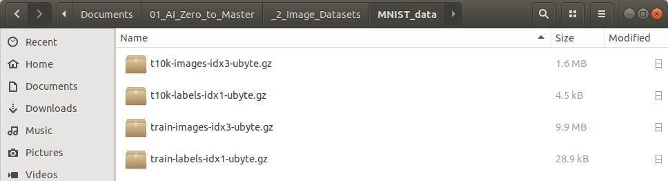
不過初次看到這個庫之後肯定是對其長相産生許多的疑問,我們從外觀上既看不到圖檔本身,也看不到任何的索引線索,他就是四個壓縮包分别名稱如下圖:
對資料庫以此方法打包的理由需要從計算機對資料的運算過程和記憶體開始說起,人類直覺的圖像是眼睛接收的光信号,這些不同顔色的光用資料的方式儲存起來後有兩種主要的格式與其對應的格式内容:
- .jpeg: height, width, channels
- .png : height, width, channels, alpha
p.s. 注意 .png 儲存格式的圖檔含有透明度的資訊,在處理圖檔的時候可以舍棄。
這些圖像使用子產品如 opencv 導入到 python 中後,是以清單的方式呈現排列的資料,并且每次令 image = cv2.imread() 這類方式把資料指向到一個 image 物件時,都是把資料存入記憶體的一個過程,在記憶體裡面的資料好處是可以非常快速的調用并處理,直到這個狀态我們才算布置完資料被丢進算法前的狀态。
然而,圖像資料導入記憶體的轉換并不是那麼的迅捷,首先必須先解析每個像素的坐标和顔色值,再把每一次讀取到的圖檔資料值合起來後,放入緩存中,這樣的流程在移動和讀取上都顯然沒有優勢,是以我們需要把資料回歸到其最基本的本質 「二進制」 上。
Binary Data 二進制資料
Reasons for using binary data 使用二進制資料的理由
如果我們手上有成批的圖檔資料,把它們傳入算法中算結果的過程就好比一個人爬上樓梯坐上滑水道的入口等待經曆一段未知的短暫旅程,滑水道有很多個通道,一次可以讓假設五個人準備滑下,而這時候如果後面遞補的人速度不夠快,就會造成該入口一定時間的空缺,直接導緻效率地下,而這個比喻中的滑水道入口代表的是深度學習 GPU 計算端口,準備下滑的人代表資料本身,而我們現在需要優化的就是如何讓 GPU 在還沒處理完這一個資料之前,就已經為它準備好下一批預處理資料,讓 GPU 永遠保持工作狀态可以進一步提升整體運算的效率,方法之一就是讓資料回歸到 「二進制」 的本質。
二進制是資料在電腦硬碟儲存狀态的原貌,也是資料被處理時最本質的狀态,是以批量圖檔資料第一件要被處理的事情就是讓他們以二進制的姿态被放入到記憶體中,此舉就好比排隊玩滑水道的人們都要事前把鞋子手表眼睛脫掉,帶着最需要的東西上去排隊後,等輪到自己時,一屁股坐上去擺好姿勢後就可以開始,沒有其他的備援動作拖慢時間。而我選擇的入門資料庫 MNIST 已經很貼心的幫我們處理好預處理的部分,分為四個類别:
- 測試集圖像資料: t10k-images-idx3-ubyte.gz
- 測試集圖像标簽: t10k-labels-idx1-ubyte.gz
- 訓練集圖像資料: train-images-idx3-ubyte.gz
- 訓練集圖像标簽: train-labels-idx1-ubyte.gz
圖像識别基本上都是屬于機器學習中的監督學習門類,是以四個類别其中兩個是對應圖檔集的标簽集,都是使用二進制的方法儲存檔案。
The approach to load images 讀取資料的方法
既然知道了資料庫裡面的結構是二進制資料,接下來就可以使用 python 裡面的子產品包解析資料,壓縮檔案為 .gz 是以對應到打開此檔案類型的子產品名為 gzip,代碼如下:
Code[1]
import gzip, os
import numpy as np

location = input('The directory of MNIST dataset: ')
path = os.path.join(location, 'train-images-idx3-ubyte.gz')
try:
    with gzip.open(path, 'rb') as fi:
        data_i = np.frombuffer(fi.read(), dtype=np.int8, offset=16)
        images_flat_all = data_i.reshape(-1, 784)
        print(images_flat_all)
        print('----- Separation -----')
        print('Size of images_flat: ', len(images_flat_all))
except:
    print("The file directory doesn't exist!")
複制
The directory of MNIST dataset: /Users/kcl/Documents/Python_Projects/01_AI_Zero_to_Master/_2_Image_Datasets/MNIST_data
[[0 0 0 ... 0 0 0]
[0 0 0 ... 0 0 0]
[0 0 0 ... 0 0 0]
...
[0 0 0 ... 0 0 0]
[0 0 0 ... 0 0 0]
[0 0 0 ... 0 0 0]]
----- Separation -----
Size of images_flat:  60000
複制
Code[2]
path_label = os.path.join(location, 'train-labels-idx1-ubyte.gz')
with gzip.open(path_label, 'rb') as fl:
    data_l = np.frombuffer(fl.read(), dtype=np.int8, offset=8)

print(data_l)
print('----- Separation -----')
print('Size of images_labels: ', len(data_l), type(data_l[0]))
複制
[5 0 4 ... 5 6 8]
----- Separation -----
Size of images_labels:  60000 <class 'numpy.int8'>
複制
代碼分為上下半段,上半段的代碼用來提取 MNIST DATASET 中訓練集的六萬個圖像樣本,每一個樣本都是由 28×28 尺寸的圖檔資料拉直成一個 1×784 長度的向量形式記錄下來;下半段的代碼則是提取對應訓練集圖像的标簽,表示每一個圖檔所描繪的數字實際上是多少,同樣也是六萬個标簽。
p.s. 資料儲存格式同理測試集與其他種類資料庫
Explanation to the code 代碼說明
基于我們對神經網絡的了解,一張圖檔被用來放入神經網絡解析的時候,需要把一個代表圖像之二維矩陣的每條 row 拼成一個長條的一維向量,以此一向量作為一張圖檔的計量機關。而 MNIST 進一步把六萬張圖檔的一維向量拼起來,形成一個超級長的向量後,以二進制的方式儲存在電腦中,是以如果要讓人們可以圖像化的看懂内部資料,就需要下面步驟還原資料:
- 使用 gzip.open 的 'rb' 讀取二進制模式打開指定的壓縮檔案
- 為了轉換資料成為 np.array ,使用 .frombuffer
- 原本的二進制資料格式使用 dtype 修改成人類讀得懂的八進制格式
- MNIST 原始資料中直到第十六位數才開始描述圖像資訊,而資料标簽則是第八位就開始描述資訊,是以 offset 設定從第十六或是八位開始讀取
- 讀出來的資料是一整條六萬個向量拼起來的資料,是以需要重新拼接資料, .reshape(-1, 784) 中的 -1 像一個未知數一樣,資料整形的過程中,隻要 column = 784,那 row 是多少就是多少
- 剝離出對應的标簽時,最後還需要對其使用 one_hot() 資料的轉換,讓标簽以例如 [0, 0, 0, 1, 0, 0, 0, 0, 0, 0] 的形式表示 "3" 的意思,目的是友善套入損失函數中運算,并尋找最優解
把資料使用 numpy 數組描述好處是處理效率高,且此庫和大多數資料處理的庫都相容,不論是便利性和效率都是很大的優勢。後面兩個連結 "numpy.frombuffer"、"在NumPy中使用動态數組" 進一步深入的講述了函數的用法。
Linear Model 線性模型
在了解資料集的資料格式和調用方法後,接下來就是把最簡單的線性模型應用到資料集中,并經過多次的梯度下降算法疊代,找出我們為此模型定義的損失函數最小值。
回顧第一章的内容,一個線性函數的代碼如下:
Code[3]
# import numpy as np
# import tensorflow as tf

# x_data = np.random.rand(100).astype(np.float32)
# y_data = x_data * 0.1 + 0.3

# weight = tf.Variable(tf.random_uniform(shape=[1], minval=-1.0, maxval=1.0))
# bias = tf.Variable(tf.zeros(shape=[1]))
# y = weight * x_data + bias

# loss = tf.reduce_mean(tf.square(y - y_data))
# optimizer = tf.train.GradientDescentOptimizer(0.5)
# training = optimizer.minimize(loss)

# sess = tf.Session()
# init = tf.global_variables_initializer()
# sess.run(init)

# for step in range(101):
#     sess.run(training)
#     if step % 10 == 0:
#         print('Round {}, weight: {}, bias: {}'
#               .format(step, sess.run(weight[0]), sess.run(bias[0])))
複制
其中我們可以看到沿着 x 軸上對應的 y 有兩組解,其中的 y_data 是我們預設的正解,而另外一個由 wx + b 計算産生的 y 則是我們要用來拟合正解的未知解,對應同一樣東西 x 的兩個不同的 y 軸值接下來需要被套入一個標明的損失函數中,上面選中的是方差法,使用該方法算出損失函數後接着用 reduce_mean() 取平均,然後使用梯度下降算法把該值降到盡可能低的地步。
同理圖像資料的歸類問題,圖檔的每一個像素資料就好比一次上面計算的過程,如同 x 的角色,是正确标簽和預測标簽所共享的一個次元資料,而 y_data 所對應的則是正确的标簽,預測的标簽則是經過一系列線性加法乘法與歸一化運算處理後才得出來的結果。
圖像資料有一點在計算上看起來不同上面示例的地方是: 每一個像素的計算被統一包含進了一個大的矩陣中,被作為整體運算的其中一個小單元平行處理,大大的加速整體運算的程序。但是計算機處理物件的緩存是有限的,我們需要适量的把圖像資料放入緩存中做平行處理,如果過載了則整個計算架構就會崩潰。
MNIST in Linear Model
梳理了一遍線性模型與 MNIST 資料集的組成元素後,接下來就是基于 Tensorflow 搭建一個線性回歸的手寫數字識别算法,有以下幾點需要重新聲明:
- batch size: 每一批次訓練圖檔的數量需要調控以免記憶體不夠
- loss function: 損失函數的原理是計算預測和實際答案之間的差距
接下來就是制定訓練步驟:
- 需要一個很簡單友善的方法呼叫我們需要的 MNIST 資料,是以需要寫一個類
- 開始搭建 Tensorflow 資料流圖,用節點設計一個 wx + b 的線性運算
- 把運算結果和實際标簽帶入損失函數中求出損失值
- 使用梯度下降法求出損失值的最小值
- 疊代訓練後,檢視訓練結果的準确率
- 檢查錯誤判斷的圖檔被歸類成了什麼标簽
Code[4]
import gzip, os
import numpy as np

################ Step No.1 to well manage the dataset. ################
class MNIST:
    # Images size is told in the official website 28*28 px.
    image_size = 28
    image_size_flat = image_size * image_size

    # Let the validation set flexible when making an instance.
    def __init__(self, val_ratio=0.1, data_dir='MNIST_data'):
        self.val_ratio = val_ratio
        self.data_dir = data_dir

        # Load 4 files to individual lists with one string pixels.
        img_train = self.load_flat_images('train-images-idx3-ubyte.gz')
        lab_train = self.load_labels('train-labels-idx1-ubyte.gz')
        img_test = self.load_flat_images('t10k-images-idx3-ubyte.gz')
        lab_test = self.load_labels('t10k-labels-idx1-ubyte.gz')

        # Determine the actual number of training / validation sets.
        self.val_train_num = round(len(img_train) * self.val_ratio)
        self.main_train_num = len(img_train) - self.val_train_num

        # The normalized image pixels value can be more convenient when training.
        # dtype=np.int64 would be more general when applying to Tensorflow.
        self.img_train = img_train[0:self.main_train_num] / 255.0
        self.lab_train = lab_train[0:self.main_train_num].astype(np.int)
        self.img_train_val = img_train[self.main_train_num:] / 255.0
        self.lab_train_val = lab_train[self.main_train_num:].astype(np.int)

        # Also convert the format of testing set.
        self.img_test = img_test / 255.0
        self.lab_test = lab_test.astype(np.int)

    # Extract the same codes from "load_flat_images" and "load_labels".
    # This method won't be called during training procedure.
    def load_binary_to_num(self, dataset_name, offset):
        path = os.path.join(self.data_dir, dataset_name)
        with gzip.open(path, 'rb') as binary_file:
            # The datasets files are stored in 8 bites, mind the format.
            data = np.frombuffer(binary_file.read(), np.uint8, offset=offset)
        return data

    # This method won't be called during training procedure.
    def load_flat_images(self, dataset_name):
        # Images offset position is 16 by default format
        data = self.load_binary_to_num(dataset_name, offset=16)
        images_flat_all = data.reshape(-1, self.image_size_flat)
        return images_flat_all

    # This method won't be called during training procedure.
    def load_labels(self, dataset_name):
        # Labels offset position is 8 by default format.
        labels_all = self.load_binary_to_num(dataset_name, offset=8)
        return labels_all

    # This method would be called for training usage.
    def one_hot(self, labels):
        # Properly use numpy module to mimic the one hot effect.
        class_num = np.max(self.lab_test) + 1
        convert = np.eye(class_num, dtype=float)[labels]
        return convert
#---------------------------------------------------------------------#

path = input("The directory of MNIST dataset: ")
data = MNIST(val_ratio=0.1, data_dir=path)
複制
The directory of MNIST dataset: /Users/kcl/Documents/Python_Projects/01_AI_Zero_to_Master/_2_Image_Datasets/MNIST_data 複制
Code[5]
import tensorflow as tf
from tqdm import tqdm

flat_size = data.image_size_flat
label_num = np.max(data.lab_test) + 1

################ Step No.2 to construct tensor graph. ################
x_train= tf.placeholder(dtype=tf.float32, shape=[None, flat_size])
t_label_oh = tf.placeholder(dtype=tf.float32, shape=[None, label_num])
t_label = tf.placeholder(dtype=tf.int64, shape=[None])

################ These are the values ################
# Initialize the beginning weights and biases by random_normal method.
weights = tf.Variable(tf.random_normal([flat_size, label_num],
                                       mean=10.0, stddev=1.0,
                                       dtype=tf.float32))
biases = tf.Variable(tf.random_normal([label_num], mean=0.0, stddev=1.0,
                                      dtype=tf.float32))
########### that we wish to get by training ##########

logits = tf.matmul(x_train, weights) + biases    # < Annotation No.1 >
# Shrink the distances between values into 0 to 1 by softmax formula.
p_label_soh = tf.nn.softmax(logits)
# Pick the position of largest value along y axis.
p_label = tf.argmax(p_label_soh, axis=1)
#---------------------------------------------------------------------#

####### Step No.3 to get a loss value by certain loss function. #######
# This softmax function can not accept input being "softmaxed" before.
CE = tf.nn.softmax_cross_entropy_with_logits_v2(logits=logits, labels=t_label_oh)
# Shrink all loss values in a matrix to only one averaged loss.
loss = tf.reduce_mean(CE)
#---------------------------------------------------------------------#

#### Step No.4 get a minimized loss value using gradient descent. ####
# Decrease this only averaged loss to a minimum value by using gradient descent.
optimizer = tf.train.AdamOptimizer(learning_rate=0.05).minimize(loss)
#---------------------------------------------------------------------#

# First return a boolean list values by tf.equal function
correct_predict = tf.equal(p_label, t_label)
# And cast them into 0 and 1 values so that its average value would be accuracy.
accuracy = tf.reduce_mean(tf.cast(correct_predict, dtype=tf.float32))

sess = tf.Session()
sess.run(tf.global_variables_initializer())

###### Step No.5 iterate the training set and check the accuracy. #####
# The trigger to train the linear model with a defined cycles.
def optimize(iteration, batch_size=32):
    for i in tqdm(range(iteration)):
        total = len(data.lab_train)
        random = np.random.randint(0, total, size=batch_size)

        # Randomly pick training images / labels with a defined batch size.
        x_train_batch = data.img_train[random]
        t_label_batch_oh = data.one_hot(data.lab_train[random])

        batch_dict = {
            x_train: x_train_batch,
            t_label_oh: t_label_batch_oh
        }

        sess.run(optimizer, feed_dict=batch_dict)

# The trigger to check the current accuracy value
def Accuracy():
    # Use the totally separate dataset to test the trained model
    test_dict = {
        x_train: data.img_test,
        t_label_oh: data.one_hot(data.lab_test),
        t_label: data.lab_test
    }

    Acc = sess.run(accuracy, feed_dict=test_dict)
    print('Accuracy on Test Set: {0:.2%}'.format(Acc))
#---------------------------------------------------------------------#

### Step No.6 plot wrong predicted pictures with its predicted label.##
import matplotlib.pyplot as plt

# We can decide how many wrong predicted images are going to be shown up.
# We can focus on the specific wrong predicted labels
def wrong_predicted_images(pic_num=[3, 4], label_number=None):
    test_dict = {
            x_train: data.img_test,
            t_label_oh: data.one_hot(data.lab_test),
            t_label: data.lab_test
        }

    correct_pred, p_lab = sess.run([correct_predict, p_label],
                                   feed_dict=test_dict)

    # To reverse the boolean value in order to pick up wrong labels
    wrong_pred = (correct_pred == False)

    # Pick up the wrong doing elements from the corresponding places
    wrong_img_test = data.img_test[wrong_pred]
    wrong_t_label = data.lab_test[wrong_pred]
    wrong_p_label = p_lab[wrong_pred]

    fig, axes = plt.subplots(pic_num[0], pic_num[1])
    fig.subplots_adjust(hspace=0.3, wspace=0.3)

    edge = data.image_size
    for ax in axes.flat:
        # If we were not interested in certain label number,
        # pick up the wrong predicted images randomly.
        if label_number is None:
            i = np.random.randint(0, len(wrong_t_label),
                                  size=None, dtype=np.int)
            pic = wrong_img_test[i].reshape(edge, edge)
            ax.imshow(pic, cmap='binary')
            xlabel = "True: {0}, Pred: {1}".format(wrong_t_label[i],
                                                   wrong_p_label[i])
        # If we are interested in certain label number,
        # pick up the specific wrong images number randomly.
        else:
            # Mind that np.where return a "tuple" that should be indexing.
            specific_idx = np.where(wrong_t_label==label_number)[0]
            i = np.random.randint(0, len(specific_idx),
                                  size=None, dtype=np.int)
            pic = wrong_img_test[specific_idx[i]].reshape(edge, edge)
            ax.imshow(pic, cmap='binary')
            xlabel = "True: {0}, Pred: {1}".format(wrong_t_label[specific_idx[i]],
                                                   wrong_p_label[specific_idx[i]])

        ax.set_xlabel(xlabel)
        # Pictures don't need any ticks, so we remove them in both dimensions
        ax.set_xticks([])
        ax.set_yticks([])

    plt.show()
#---------------------------------------------------------------------#
複制
/Library/Frameworks/Python.framework/Versions/3.6/lib/python3.6/importlib/_bootstrap.py:205: RuntimeWarning: compiletime version 3.5 of module 'tensorflow.python.framework.fast_tensor_util' does not match runtime version 3.6
  return f(*args, **kwds)
/Library/Frameworks/Python.framework/Versions/3.6/lib/python3.6/site-packages/h5py/__init__.py:36: FutureWarning: Conversion of the second argument of issubdtype from `float` to `np.floating` is deprecated. In future, it will be treated as `np.float64 == np.dtype(float).type`.
  from ._conv import register_converters as _register_converters
複制
Code[6]
print(x_train.shape)
Accuracy()        # Accuracy before doing anything
optimize(10)
Accuracy()        # Iterate 10 times
optimize(1000)
Accuracy()        # Iterate 10 + 1000 times
optimize(10000)
Accuracy()        # Iterate 10 + 1000 + 10000 times
複制
(?, 784)
Accuracy on Test Set: 10.58%
Accuracy on Test Set: 48.68%
100%|██████████| 1000/1000 [00:00<00:00, 1424.39it/s]
  2%|▏            | 152/10000 [00:00<00:06, 1516.28it/s]
Accuracy on Test Set: 86.83%
100%|██████████| 10000/10000 [00:06<00:00, 1473.50it/s]
Accuracy on Test Set: 88.52%
複制
Annotation No.1 tf.matmul(x_train, weights)
這個環節是在了解整個神經網絡訓練原理後,最重要的一個子标題,計算的矩陣模型中必須兼顧 random_batch 提取随意多的資料集,同時符合矩陣乘法的運算原理,如下圖描述:

矩陣位置前後順序很重要,由于資料集本身經過我們處理後,就是左邊矩陣的格式,在期望輸出為右邊矩陣的情況下,隻能是 x·w 的順序,以 x 的随機列數來決定後面預測的标簽列數, w 則決定有幾個歸類标簽。
Reason of using one_hot()
資料集經過一番線性運算後得出的結果如上圖所見,隻能是 size=[None, 10] 的大小,但是資料集給的标簽答案是數字本身,是以我們需要一個手段把數字轉換成 10 個元素組成的向量,而第一選擇方法就是 one_hot() ,同時使用 one_hot 的結果來計算損失函數。
Code[7]
wrong_predicted_images(pic_num=[3, 3], label_number=5) 複制
Code[8]
wrong_predicted_images(pic_num=[3, 3], label_number=4) 複制
Code[9]
# When everything is done above, mind to execute the line below.
# It will help us to release occupied memory in our computer.
sess.close()
複制