目的:what to transfer,以及如何有效避免negative transfer上。
假設:所有的域之間有着公有的特征(Shared)和私有的特征(Private),如果将各個域的私有特征也進行遷移的話就會造成負遷移(negative transfer)。
基于此,提出了Domain Separation Networks(DSNs)。
Domain Separation Networks (DSNs)
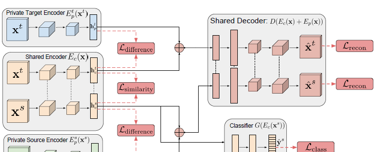
網絡結構包含:
- Shared Encoder E c ( x ) E_{c}(x) Ec(x): 提取共有特征,使得不同域之間遷移。
- Private Source Encoder E p s ( x s ) E_{p}^{s}(x^{s}) Eps(xs) : 源域私有編碼器, 用于提取源域資料私有特征。
- Private Target Encoder E p t ( x t ) E_{p}^{t}(x^{t}) Ept(xt): 目标域私有編碼器,用來提取目标域的私有特征。
- Shared Decoder: 共享的解碼器,輸入時私有特征和共有特征,用于重構圖像。
- 源域分類器 G ( E c ( x s ) ) G\left(E_{c}\left(x^{s}\right)\right) G(Ec(xs)): 源域資料的分類器,輸入是公有特征。訓練完成之後,可以用來對目标域資料上分類。
其中, x s , x t x^s, x^t xs,xt分别表示源域和目标域輸入,通過公有和私有編碼器之後,分别輸出 h p s , h c s h_p^s, h_c^s hps,hcs、 對應源域私有特征和共有特征, h p t , h c t h_p^t, h_c^t hpt,hct,對應目标域特征。
Loss
difference loss
為什麼 E p t ( x ) , E p s ( x ) E_p^t(x), E_p^s(x) Ept(x),Eps(x)就能輸出私有特征呢?
作者損失函數層面進行了限制,定義差異損失:
L difference = ∥ H c s ⊤ H p s ∥ F 2 + ∥ H c t ⊤ H p t ∥ F 2 \mathcal{L}_{\text {difference }}=\left\|\mathbf{H}_{c}^{s \top} \mathbf{H}_{p}^{s}\right\|_{F}^{2}+\left\|\mathbf{H}_{c}^{t^{\top}} \mathbf{H}_{p}^{t}\right\|_{F}^{2} Ldifference =∥∥Hcs⊤Hps∥∥F2+∥∥∥Hct⊤Hpt∥∥∥F2
∥ ⋅ ∥ F 2 \|\cdot\|_{F}^{2} ∥⋅∥F2表示矩陣範式,而中間是 H c s ⊤ H p s \mathbf{H}_{c}^{\mathbf{s} \top} \mathbf{H}_{p}^{s} Hcs⊤Hps,隻有兩個矩陣正交,範式才為0,是以這個損失鼓勵私有特征和共有特征不相似,正交的時候最小。
Similarity loss
為什麼 E c ( x ) E_c(x) Ec(x)就能輸出共有特征?
為了保證源域和目标域是可遷移的,就要保證 h c t , h c s h_c^t, h_c^s hct,hcs的分布相似性。
注意是 h c t , h c s h_c^t, h_c^s hct,hcs的分布相似性,非向量相似性,因為本來就是不同輸入,不能适得其輸出相似。
作者用到了Gradient Reversal Layer (GRL):
簡單講就是找到一個函數Q(f(u)),使得梯度取反:
d d u Q ( f ( u ) ) = − d d u f ( u ) \frac{d}{d \mathbf{u}} Q(f(\mathbf{u}))=-\frac{d}{d \mathbf{u}} f(\mathbf{u}) dudQ(f(u))=−dudf(u)
損失函數:
L similarity D A N N = ∑ i = 0 N s + N t { d i log d ^ i + ( 1 − d i ) log ( 1 − d ^ i ) } \mathcal{L}_{\text {similarity }}^{\mathrm{DANN}}=\sum_{i=0}^{N_{s}+N_{t}}\left\{d_{i} \log \hat{d}_{i}+\left(1-d_{i}\right) \log \left(1-\hat{d}_{i}\right)\right\} Lsimilarity DANN=i=0∑Ns+Nt{dilogd^i+(1−di)log(1−d^i)}
使用了對抗學習的思想,通過一個域分類器 Z ( Q ( h c ) ; θ z ) , h c = E c ( x ; θ c ) Z\left(Q\left(\mathbf{h}_{c}\right) ; \boldsymbol{\theta}_{z}\right), \mathbf{h}_{c}=E_{c}\left(\mathbf{x} ; \boldsymbol{\theta}_{c}\right) Z(Q(hc);θz),hc=Ec(x;θc),來區分 h c t , h c s h_c^t, h_c^s hct,hcs是屬于源域還是目标域。對于分類器的參數 θ z \theta_z θz通過梯度求導來最小化分類損失,讓分類器分的更準。而通過加入Q,來使用GRL,使得在優化 θ c \theta_c θc的時候讓分類器無法分辨輸入屬于source還是target。
Reconstruction loss
怎麼保證 h p s , h p t , h c s , h c t h_{p}^{s}, h_{p}^{t}, h_{c}^{s},h_{c}^{t} hps,hpt,hcs,hct都是有意義的呢?例如 h p s = 0 , h p t = 0 , h c s = h c t = 1 h_{p}^{s}=0, \quad h_{p}^{t}=0, \quad h_{c}^{s}=h_{c}^{t}=1 hps=0,hpt=0,hcs=hct=1的時候,上述損失就可以達到0.
是以作者引入了重構損失。
(3) L recon = ∑ i = 1 N s L si − mse ( x i s , x ^ i s ) + ∑ i = 1 N t L s i − mse ( x i t , x ^ i t ) L s i − m s e ( x , x ^ ) = 1 k ∥ x − x ^ ∥ 2 2 − 1 k 2 ( [ x − x ^ ] ⋅ 1 k ) 2 \mathcal{L}_{\text {recon }}=\sum_{i=1}^{N_{s}} \mathcal{L}_{\text {si }_{-} \text {mse }}\left(\mathrm{x}_{i}^{s}, \hat{\mathrm{x}}_{i}^{s}\right)+\sum_{i=1}^{N_{t}} \mathcal{L}_{\mathrm{si}_{-} \text {mse }}\left(\mathrm{x}_{i}^{t}, \hat{\mathrm{x}}_{i}^{t}\right) \tag{3} \\ \mathcal{L}_{\mathrm{si}_{-} \mathrm{mse}}(\mathrm{x}, \hat{\mathrm{x}})=\frac{1}{k}\|\mathrm{x}-\hat{\mathrm{x}}\|_{2}^{2}-\frac{1}{k^{2}}\left([\mathrm{x}-\hat{\mathrm{x}}] \cdot 1_{k}\right)^{2} Lrecon =i=1∑NsLsi −mse (xis,x^is)+i=1∑NtLsi−mse (xit,x^it)Lsi−mse(x,x^)=k1∥x−x^∥22−k21([x−x^]⋅1k)2(3)
其中k為輸入x的像素個數,1k為長度為k的向量; ∥ ⋅ ∥ 2 2 \|\cdot\|_{2}^{2} ∥⋅∥22是向量的平方模。
雖然均值平方誤差損失傳統上用于重建任務,但它會懲罰在縮放項下正确的預測。相反,尺度不變的均方誤差抵消了像素對之間的差異。這允許模型學習複制被模組化對象的整體形狀,而不需要在輸入的絕對顔色或強度上花費模組化能力。
在實驗中,作者用傳統的均方誤差損失代替式3中的尺度不變損失,驗證了這種重構損失确實是正确的選擇。
task loss
最後是分類器 G ( E c ( x s ) ) G\left(E_{c}\left(x^{s}\right)\right) G(Ec(xs))的分類損失:
L t a s k = − ∑ i = 0 N s y i s ⋅ log y ^ i s \mathcal{L}_{\mathrm{task}}=-\sum_{i=0}^{N_{s}} \mathbf{y}_{i}^{s} \cdot \log \hat{\mathbf{y}}_{i}^{s} Ltask=−i=0∑Nsyis⋅logy^is
注意分類器的輸入是共有特征,是以保證對于目标域,能夠直接遷移過來,使用此分類器做分類任務。
Expriment
作者提供四組遷移的實驗,五個資料集。Source-only表示沒有進行遷移,隻用源域資料進行訓練得到的模型的精度;Target-only表示沒有遷移,隻有帶标記的目标域資料進行訓練得到的模型的精度;中間五行表示當目标域資料無标記,進行遷移之後各個模型的精度。

可以看出,DSNs算法還是有明顯的提高。
Reference
- Domain Separation Networks.
- Domain-adversarial training of neural networks.