拓端tecdat|R語言中的copula GARCH模型拟合時間序列并模拟分析

​

 在這個文章中，我們示範了copula GARCH方法（一般情況下）。

1 模拟資料

首先，我們模拟一下創新分布。我們選擇了一個小的樣本量。理想情況下，樣本量應該更大，更容易發現GARCH效應。 

1. ## 模拟創新
2. d <- 2 # 次元
3. tau <- 0.5 # Kendall's tau
4. Copula("t", param = th, dim = d, df = nu) # 定義copula對象
5. rCopula(n, cop) # 對copula進行采樣
6. sqrt((nu.-2)/nu.) * qt(U, df = nu) # 對于ugarchpath()來說，邊緣必須具有均值0和方差1!

現在我們用這些copula依賴的創新分布來模拟兩個ARMA(1,1)-GARCH(1,1)過程。

1. ## 邊緣模型的參數
2. fixed.p <- list(mu = 1,
3. spec(varModel, meanModel,
4. fixed.pars ) # 條件創新密度（或使用，例如，"std"）
5. ## 使用創新模拟ARMA-GARCH模型
6. ## 注意: ugarchpath(): 從spec中模拟;
7. garchpath(uspec,
8. n.sim = n, # 模拟的路徑長度
9. ## 提取結果系列
10. X. <- fitted(X) # X_t = mu_t + eps_t (simulated process)
11. ## 基本檢查:
12. stopifnot(all.equal(X., X@path$seriesSim, check.attributes = FALSE),
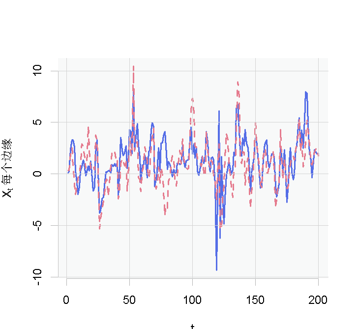
13. ## 繪制邊緣函數
14. plot(X., type = "l", xlab = "t")

2 基于模拟資料的拟合程式

我們現在展示如何對X進行ARMA(1,1)-GARCH(1,1)過程的拟合（我們删除參數fixed.pars來估計這些參數）。

1. spec(varModel, mean.model = meanModel)
2. ugarchfit(uspec, data = x))

檢查（标準化的）Z，即殘差Z的僞觀測值。 

plot(U.)
      

對于邊緣分布，我們也假定為t分布，但自由度不同。

fit("t", dim = 2), data = U., method = "mpl")
      

1. nu. <- rep(nu., d) # 邊緣自由度
2. est <- cbind(fitted = c(estimate, nu.), true = c(th, nu, nu.)) # 拟合與真實值

3 從拟合的時間序列模型進行模拟

從拟合的copula 模型進行模拟。 

1. set.seed(271) # 可重複性
2. sapply(1:d, function(j) sqrt((nu[j]-2)/nu[j]) * qt(U[,j], df = nu[j]))
3. ## => 創新必須是标準化的garch()
4. sim(fit[[j]], n.sim = n, m.sim = 1,

并繪制出每個結果序列（XtXt）。 

1. apply(sim,fitted(x)) # 模拟序列
2. plot(X.., type = "l")