基礎_cifar10_序貫

今天的基礎研究主要是在cifar10資料集上解決一下幾個問題：1、從頭開始，從最簡單的序貫開始，嘗試model的構造；

2、要将模型列印出來。最好是能夠列印出圖檔，否則也要summary;

3、嘗試對例子的參數進行分析，得出初步修改意見。

1、構模組化型

'''Train a simple deep CNN on the CIFAR10 small images dataset.

It gets to 75% validation accuracy in 25 epochs, and 79% after 50 epochs.

(it's still underfitting at that point, though).

'''

from __future__ import print_function

#!apt-get -qq install -y graphviz && pip install -q pydot

import pydot

import keras

import cv2

from keras.datasets import cifar10

from keras.preprocessing.image import ImageDataGenerator

from keras.models import Sequential

from keras.layers import Dense, Dropout, Activation, Flatten

from keras.layers import Conv2D, MaxPooling2D

from keras.utils.vis_utils import plot_model

import matplotlib.image as image # image 用于讀取圖檔

import matplotlib.pyplot as plt

import os

%matplotlib inline

%config InlineBackend.figure_format = 'retina'

batch_size = 32

num_classes = 10

#epochs = 100

epochs = 3

data_augmentation = True

num_predictions = 20

save_dir = os.path.join(os.getcwd(), 'saved_models')

model_name = 'keras_cifar10_trained_model.h5'

# The data, split between train and test sets:

(x_train, y_train), (x_test, y_test) = cifar10.load_data()

print('x_train shape:', x_train.shape)

print(x_train.shape[0], 'train samples')

print(x_test.shape[0], 'test samples')

# Convert class vectors to binary class matrices.

y_train = keras.utils.to_categorical(y_train, num_classes)

y_test = keras.utils.to_categorical(y_test, num_classes)

model = Sequential()

model.add(Conv2D(32, (3, 3), padding='same', input_shape=x_train.shape[1:]))model.add(Activation('relu'))model.add(Conv2D(32, (3, 3)))model.add(Activation('relu'))model.add(MaxPooling2D(pool_size=(2, 2)))model.add(Dropout(0.25))

#顯示模型

model.summary()

plot_model(model,to_file='model1111.png',show_shapes=True)

files.download('model1111.png')

img = image.imread('model1111.png')

print(img.shape)

plt.imshow(img) # 顯示圖檔

plt.axis('off') # 不顯示坐标軸

plt.show()

# initiate RMSprop optimizer

opt = keras.optimizers.rmsprop(lr=0.0001, decay=1e-6)

# Let's train the model using RMSprop

model.compile(loss='categorical_crossentropy',

optimizer=opt,

metrics=['accuracy'])

x_train = x_train.astype('float32')

x_test = x_test.astype('float32')

x_train /= 255

x_test /= 255

if not data_augmentation:

print('Not using data augmentation.')

model.fit(x_train, y_train,

batch_size=batch_size,

epochs=epochs,

validation_data=(x_test, y_test),

shuffle=True)

else:

print('Using real-time data augmentation.')

# This will do preprocessing and realtime data augmentation:

datagen = ImageDataGenerator(

featurewise_center=False, # set input mean to 0 over the dataset

samplewise_center=False, # set each sample mean to 0

featurewise_std_normalization=False, # divide inputs by std of the dataset

samplewise_std_normalization=False, # divide each input by its std

zca_whitening=False, # apply ZCA whitening

rotation_range=0, # randomly rotate images in the range (degrees, 0 to 180)

width_shift_range=0.1, # randomly shift images horizontally (fraction of total width)

height_shift_range=0.1, # randomly shift images vertically (fraction of total height)

horizontal_flip=True, # randomly flip images

vertical_flip=False) # randomly flip images

# Compute quantities required for feature-wise normalization

# (std, mean, and principal components if ZCA whitening is applied).

datagen.fit(x_train)

# Fit the model on the batches generated by datagen.flow().

model.fit_generator(datagen.flow(x_train, y_train,

batch_size=batch_size),

epochs=epochs,

validation_data=(x_test, y_test),

workers=4)

# Save model and weights

if not os.path.isdir(save_dir):

os.makedirs(save_dir)

model_path = os.path.join(save_dir, model_name)

model.save(model_path)

print('Saved trained model at %s ' % model_path)

# Score trained model.

scores = model.evaluate(x_test, y_test, verbose=1)

print('Test loss:', scores[0])

print('Test accuracy:', scores[1])

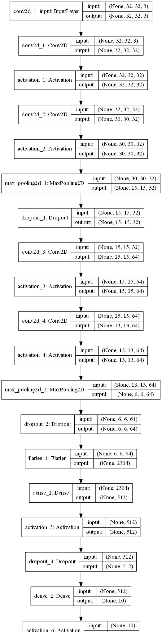
2、要将模型列印出來，目前隻有本地才有圖檔。這個圖檔也可以本地看。

Using TensorFlow backend.

x_train shape: (50000, 32, 32, 3)

50000 train samples

10000 test samples

_________________________________________________________________

Layer (type)                 Output Shape              Param #  

=================================================================

conv2d_1 (Conv2D)            (None, 32, 32, 32)        896      

activation_1 (Activation)    (None, 32, 32, 32)        0        

conv2d_2 (Conv2D)            (None, 30, 30, 32)        9248     

activation_2 (Activation)    (None, 30, 30, 32)        0        

max_pooling2d_1 (MaxPooling2 (None, 15, 15, 32)        0        

dropout_1 (Dropout)          (None, 15, 15, 32)        0        

conv2d_3 (Conv2D)            (None, 15, 15, 64)        18496    

activation_3 (Activation)    (None, 15, 15, 64)        0        

conv2d_4 (Conv2D)            (None, 13, 13, 64)        36928    

activation_4 (Activation)    (None, 13, 13, 64)        0        

max_pooling2d_2 (MaxPooling2 (None, 6, 6, 64)          0        

dropout_2 (Dropout)          (None, 6, 6, 64)          0        

flatten_1 (Flatten)          (None, 2304)              0        

dense_1 (Dense)              (None, 512)               1180160  

activation_5 (Activation)    (None, 512)               0        

dropout_3 (Dropout)          (None, 512)               0        

dense_2 (Dense)              (None, 10)                5130     

activation_6 (Activation)    (None, 10)                0        

Total params: 1,250,858

Trainable params: 1,250,858

Non-trainable params: 0

(2065, 635, 4)

Using real-time data augmentation.

WARNING:tensorflow:Variable *= will be deprecated. Use variable.assign_mul if you want assignment to the variable value or 'x = x * y' if you want a new python Tensor object.

Epoch 1/3

138/1563 [=>........大圖：

3、嘗試對例子的參數進行分析，得出初步修改意見

。

從這個序貫模型的建立過程中，其模型大概是這樣的：

第一段是

model.add(Conv2D(32, (3, 3), padding='same',input_shape=x_train.shape[1:]))

model.add(Activation('relu'))

model.add(Conv2D(32, (3, 3)))

model.add(MaxPooling2D(pool_size=(2, 2)))

model.add(Dropout(0.25))

基本上相當于卷積->激活->卷積->激活->maxPooling->dropout

然後

model.add(Conv2D(64, (3, 3), padding='same'))

model.add(Conv2D(64, (3, 3)))

幾乎是原樣的來了一遍，唯一不同的是變成了64個一組。

model.add(Flatten())

model.add(Dense(512))

model.add(Dropout(0.5))

model.add(Dense(num_classes))

model.add(Activation('softmax'))

最後，到輸出階段了，應該是要準備輸出了。

在這個地方，應該觸及DL這門技術的核心了，就是我應該構造增益的網絡？又怎樣根據生成的結果來調整網絡。遷移我在圖像處理方面的知識，我首先是知道了基礎的工具，然後有了很多實際的經驗，這樣才能夠在拿到問題的第一時間，有初步的設想。

更簡單的網絡代表可以更快 地訓練，在我的研究過程中，需要尋找的并不是我們的網絡能夠複雜到什麼程度—而是怎樣簡單的網絡就可以完成目标，達到既定的acc。首先可能是90%到95%，逐漸地去接觸更多東西。在cifar-10上要起碼達到這個結果。

當然我知道增加epoch，一般時候能夠提高準确率，當然也會過拟合；另一個方向，如果我縮小資料，比如在上面的例子中，不添加64位層，結果是這樣：

model = Sequential() model.add(Conv2D(32, (3, 3), padding='same',                  input_shape=x_train.shape[1:])) model.add(Activation('relu')) model.add(Conv2D(32, (3, 3))) model.add(Activation('relu')) model.add(MaxPooling2D(pool_size=(2, 2))) model.add(Dropout(0.25)) model.add(Conv2D(64, (3, 3), padding='same')) model.add(Activation('relu')) model.add(Conv2D(64, (3, 3))) model.add(Activation('relu')) model.add(MaxPooling2D(pool_size=(2, 2))) model.add(Dropout(0.25)) model.add(Flatten()) model.add(Dense(512)) model.add(Activation('relu')) model.add(Dropout(0.5)) model.add(Dense(num_classes)) model.add(Activation('softmax')) model2 = Sequential() model2.add(Conv2D(32, (3, 3), padding='same',                  input_shape=x_train.shape[1:])) model2.add(Activation('relu')) model2.add(Conv2D(32, (3, 3))) model2.add(Activation('relu')) model2.add(MaxPooling2D(pool_size=(2, 2))) model2.add(Dropout(0.25)) model2.add(Flatten()) model2.add(Dense(512)) model2.add(Activation('relu')) model2.add(Dropout(0.5)) model2.add(Dense(num_classes)) model2.add(Activation('softmax'))

Test loss: 0.8056231224060059

Test accuracy: 0.7182

10000/10000 [==============================] - 2s 161us/step

Test loss2: 0.9484411451339722

Test accuracy2: 0.6764

最後，在《NN&DL》中反複被提及的一點，我也實際體會到了：訓練需要時間，你可以先去做其它的事情。

到此，我認為《基礎_cifar10_序貫》可以結束。

來自為知筆記(Wiz)

目前方向：圖像拼接融合、圖像識别

聯系方式：[email protected]