Adversarial Training with Rectified Rejection

目錄

概

主要内容

rejection

實際使用

代碼

Pang T., Zhang H., He D., Dong Y., Su H., Chen W., Zhu J., Liu T. Adversarial training with rectified rejection. arXiv Preprint, arXiv: 2105.14785, 2021.

通過對置信度進行矯正, 然後再根據threshold (1/2)判斷是否拒絕. 有點detection的味道, 總體來說是很有趣的點子.

假設一個網絡\(f_{\theta}\) 将樣本\(x\)映射為機率向量\(f_{\theta}(x)\), 則其置信度(confidence)為

\[f_{\theta}(x)[y^m], y^m := \mathop{\arg\max} \limits_{k} f_{\theta}(x)[k],

\]

若該樣本的真實的标簽為\(y\), 進一步定義真實的置信度\(\text{T-Con}\)為

\[f_{\theta}(x)[y].

我們進一步定義一個分類器\(F\):

\[F(x) =

\left \{

\begin{array}{ll}

y^m & \text{if } f_{\theta}(x)[y] \ge \frac{1}{2}, \\

\text{don't know} & \text{if } f_{\theta}(x)[y] < \frac{1}{2}.

\end{array}

\right .

顯然這種情況下, 就算\(f\)訓練得再糟糕, \(F\)都不會分錯(雖然可能大部分都是拒絕判斷, 但是拒絕判斷在面對對抗樣本的時候是有用的).

但是上面的情況是必須知道樣本标簽\(y\)的, 都知道标簽了還弄個分類器不是多次一舉. 是以我們現在要做的, 是做一個近似

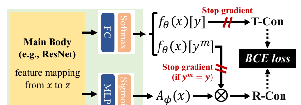
如上圖所示, 我們要通過一個近似的\(\text{R-Con}\)來代替\(\text{T-Con}\), Rectified Confidence通過如下的方式建構:

通過encoder将\(x\)映為特征\(z\);

\(z\)通過全連接配接層和softmax層獲得機率向量\(f_{\theta}(x)\);

\(z\)通過MLP和sigmoid層獲得\(A_{\phi}(x) \in [0, 1]\);

計算Rectified Confidence:

\[\text{R-Con}(x) = f_{\theta}(x)[y^m]A_{\phi}(x).

顯然, 若要\(\text{R-Con}(x) = \text{T-Con}(x)\), 則有

\[A_{\phi}(x) = A_{\phi}^*(x) = \frac{f_{\theta}(x)[y]}{f_{\theta}(x)[y^m]}.

為此, 通過BCE損失:

\[\mathcal{L}_{RR}(x, y;\theta, \phi)

= \mathbf{BCE}(f_{\theta}(x)[y^m]A_{\phi}(x) \| f_{\theta}(x)[y]) \\

\mathbf{BCE}(f\|g) = g \cdot \log f + (1 - g) \cdot \log (1 - f).

故總的損失為:

\[\min_{\theta, \phi}\: \mathbb{E}_{p(x y)}[\mathcal{L}_T(x^*, y;\theta) + \lambda \mathcal{L}_{RR}(x^*, y; \theta, \phi)], \\

x^* = \mathop{\arg \max} \limits_{x' \in B(x)} \mathcal{L}_{A}(x', y; \theta).

注意圖中的stop gradient部分, 最上面是為了一個單向的趨近(雖然encoder部分是會依然交涉), 第二個部分作者覺得當\(y^m = y\)時, 該樣本比較簡單, 而對抗學習應該注中難的樣本, 這樣不容易陷入局部最優, 經驗之談吧.

y^m & \text{if } \text{R-Con}(x) \ge \frac{1}{2}, \\

\text{don't know} & \text{if } \text{R-Con}(x) < \frac{1}{2}.

現在的疑問是, 什麼時候這個分類器是沒有錯判的.

定義: 當下列界,

\(|\log (\frac{A_{\phi}(x)}{A_{\phi}^*(x)})| \le \log (\frac{2}{2-\xi})\);

\(|A_{\phi}(x) - A_{\phi}^*(x)| \le \frac{\xi}{2}\)

至少一個成立時, 稱\(A_{\phi}(x)\)在點\(x\)處為\(\xi\text{-error}\), \(\xi \in [0, 1)\).

定理1: 假設\(x_+, x_-\)分别為被\(f\)正判和誤判的樣本, 即

\[y_+^m = y_+, y^m_- \not = y_-,

但均滿足(即置信度足夠高)

\[f(x_+)[y_+^m] > \frac{1}{2-\xi}, \quad f(x_-)[y_-^m] > \frac{1}{2-\xi}, \: \xi \in [0, 1).

若\(A_{\phi}\)在\(x_+, x_-\)處滿足\(\xi\text{-error}\), 則\(\text{R-Con}(x_+) > \frac{1}{2} > \text{R-Con}(x_-)\), 即此時\(F(x_+)\)為正确判斷, \(F(x_-)\)拒絕判斷.

proof:

界1等價于:

\[\frac{2-\xi}{2}f(x)[y] \le \text{R-Con}(x) \le \frac{2}{2-\xi} f(x)[y],

界2等價于

\[f(x)[y] - \frac{\xi}{2} f(x)[y^m] \le \text{R-Con}(x) \le f(x)[y] + \frac{\xi}{2} f(x)[y^m].

因為

\[f(x_+)[y_+] = f(x_+)[y_+^m] > \frac{1}{2 - \xi},\\

\frac{2-\xi}{2}f(x_+)[y_+] > \frac{1}{2}, \\

f(x)[y] - \frac{\xi}{2} f(x)[y^m] = f(x)[y^m] - \frac{\xi}{2} f(x)[y^m] > \frac{1}{2}.

是以\(\text{R-Con}(x_+) > \frac{1}{2}\).

又因為

\[f(x)[y] \le 1 - f(x)[y^m] \Rightarrow f(x_-)[y_-] < \frac{1-\xi}{2-\xi}.

易證

\[\frac{2}{2-\xi}\frac{1-\xi}{2-\xi} \le \frac{1}{2}, \xi \in [0, 1),

\[f(x_-)[y_-] + \frac{\xi}{2}f(x_-)[y^m_-] \le 1 - t + \frac{\xi}{2}t < \frac{1}{2}, \quad t:= f(x_-)[y_-^m] > \frac{1}{2-\xi}.

故\(\text{R-Con}(x_-) < \frac{1}{2}\).

證畢.

在實際使用中, threshold 似乎并不是固定為1/2, 而是通過TPR-FPR曲線選擇的(TPR-95).

y^m & \text{if } \text{R-Con}(x) \ge t, \\

\text{don't know} & \text{if } \text{R-Con}(x) < t.

原文代碼