資料檔案:(汽車油耗分析都是基于這個檔案進行分析的)
下載下傳位址:https://www.fueleconomy.gov/feg/download.shtml
一、環境安裝與配置
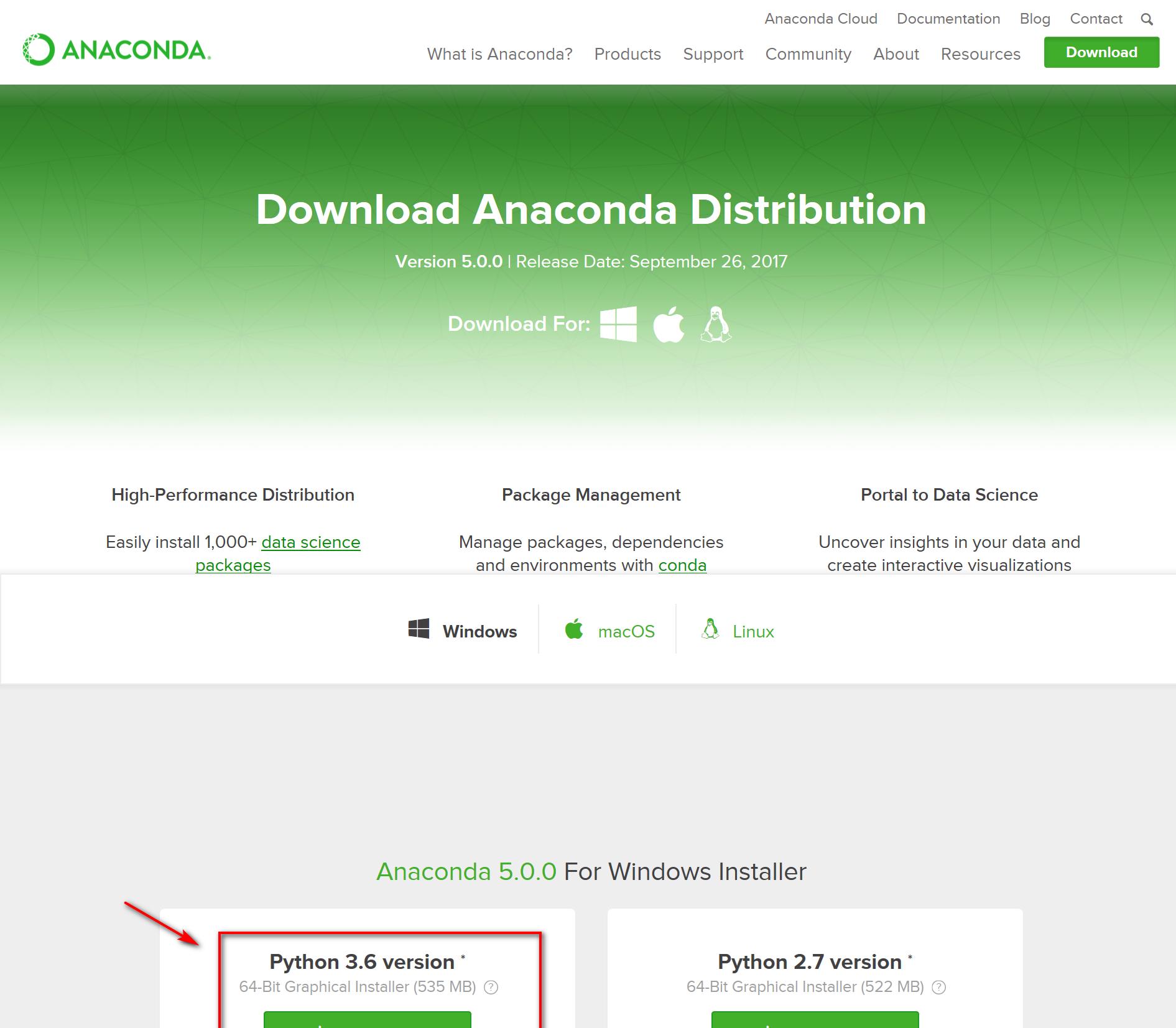
1、下載下傳安裝jupyter notebook之前 ,先下載下傳安裝anaconda(我的電腦系統:windows10,64位)官網下載下傳: https://www.anaconda.com/download/#windows
安裝成功後,打開指令行視窗,輸入【pip install jupyter】就可以下載下傳安裝jupyter,詳見步驟3。
2、下載下傳安裝python3.6.1(提前已經安裝并配置python環境),關于python的下載下傳安裝和配置可以百度,主要是配置環境變量path。安裝配置成功後,在指令行中輸入python,如圖:

3、在安裝好的Anaconda Prompt指令視窗中,輸入pip install jupyter(圖為安裝成功後指令行顯示)
4、安裝ggplot(運作代碼時報錯,發現問題後,安裝解決)
ggplot for python:ggplot是一個python的庫,基本上是對R語言ggplot的功能移植到Python上。運作安裝:pip install ggplot
5、将檔案:vehicles.csv放到磁盤目錄下:D:/model/vehicles.csv
(這裡的路徑要和代碼中此處的路徑一緻 vehicles = pd.read_csv(“D:/model/vehicles.csv”) )
二、在Jupyter Notebook中開始項目
1、打開Jupyter Notebook,建立python檔案:
在In[ ]單元格中輸入python指令:
import pandas as pd
import numpy as np
from ggplot import *
import matplotlib.pyplot as plt
%matplotlib inline
vehicles = pd.read_csv(“D:/model/vehicles.csv”)
print(vehicles.head())
按Shift+enter執行單元格代碼,結果如圖:
2、描述汽車油耗等資料:
接着上面的代碼,繼續輸入:(将之前的代碼注釋掉,簡化頁面)
(1)、檢視觀測點(行):len(vehicles)
(2)、檢視變量數(列):print (len(vehicles.columns))
print(vehicles.columns)
(3)、檢視年份資訊:print(len(pd.unique(vehicles.year)))
print(min(vehicles.year))
print(max(vehicles.year))
(4)、檢視燃料類型:print(pd.value_counts(vehicles.fuelType))
(5)、檢視變速箱類型: pd.value_counts(vehicles.trany)
trany變量自動擋是以A開頭,手動擋是以M開頭;故建立一個新變量trany2:
vehicles[‘trany2’] = vehicles.trany.str[0]
pd.value_counts(vehicles.trany2)
3、分析汽車油耗随時間變化的規律
(1)、先按年份分組:grouped = vehicles.groupby(‘year’)
再計算其中三列的均值:
averaged= grouped[‘comb08’, ‘highway08’, ‘city08’].agg([np.mean])
為友善分析,對其進行重命名,然後建立一個‘year’的列,包含該資料框data frame的索引:
averaged.columns = [‘comb08_mean’, ‘highwayo8_mean’, ‘city08_mean’]
averaged[‘year’] = averaged.index
print(averaged )
(2)、使用ggplot包将結果繪成散點圖:allCarPlt = ggplot(averaged, aes(‘year’, ‘comb08_mean’)) + geom_point(colour=’steelblue’) + xlab(“Year”) + ylab(“Average MPG”) + ggtitle(“All cars”)
print(allCarPlt)
(3)、去除混合動力汽車:
criteria1 = vehicles.fuelType1.isin([‘Regular Gasoline’, ‘Premium Gasoline’, ‘Midgrade Gasoline’])
criteria2 = vehicles.fuelType2.isnull()
criteria3 = vehicles.atvType != ‘Hybrid’
vehicles_non_hybrid = vehicles[criteria1 & criteria2 & criteria3]
将得到的資料框data frame按年份分組,并計算平均油耗:
grouped = vehicles_non_hybrid.groupby([‘year’])
averaged = grouped[‘comb08’].agg([np.mean])
averaged[‘hahhahah’] = averaged.index
print(averaged)
(4)、檢視是否大引擎的汽車越來越少:print(pd.unique(vehicles_non_hybrid.displ))
(5)、去掉nan值,并用astype方法保證各個值都是float型的:
criteria = vehicles_non_hybrid.displ.notnull()
vehicles_non_hybrid = vehicles_non_hybrid[criteria]
vehicles_non_hybrid.loc[:,’displ’] = vehicles_non_hybrid.displ.astype(‘float’)
criteria = vehicles_non_hybrid.comb08.notnull()
vehicles_non_hybrid = vehicles_non_hybrid[criteria]
vehicles_non_hybrid.loc[:,’comb08’] = vehicles_non_hybrid.comb08.astype(‘float’)
最後用ggplot包來繪圖:
gasOnlineCarsPlt = ggplot(vehicles_non_hybrid, aes(‘displ’, ‘comb08’)) + geom_point(color=’steelblue’) +xlab(‘Engine Displacement’) + ylab(‘Average MPG’) + ggtitle(‘Gasoline cars’)
print(gasOnlineCarsPlt)
(6)、檢視是否平均起來汽車越來越少了:
grouped_by_year = vehicles_non_hybrid.groupby([‘year’])
avg_grouped_by_year = grouped_by_year[‘displ’, ‘comb08’].agg([np.mean])
計算displ和conm08的均值,并改造資料框data frame:
avg_grouped_by_year[‘year’] = avg_grouped_by_year.index
melted_avg_grouped_by_year = pd.melt(avg_grouped_by_year, id_vars=’year’)
建立分屏繪圖:
p = ggplot(aes(x=’year’, y=’value’, color = ‘variable_0’), data=melted_avg_grouped_by_year)
p + geom_point() + facet_grid(“variable_0”,scales=”free”) #scales參數fixed表示固定坐标軸刻度,free表示回報坐标軸刻度
print(p)
4、調查汽車的制造商和型号
接下來的步驟會引導我們繼續深入完成資料探索
(1)、首先檢視cylinders變量有哪些可能的值:print(pd.unique(vehicles_non_hybrid.cylinders))
(2)、再将cylinders變量轉換為float類型,這樣可以輕松友善地找到data frame的子集:
vehicles_non_hybrid.cylinders = vehicles_non_hybrid.cylinders.astype(‘float’)
pd.unique(vehicles_non_hybrid.cylinders)
(3)、現在,我們可以檢視各個時間段有四缸引擎汽車的品牌數量:
vehicles_non_hybrid_4 = vehicles_non_hybrid[(vehicles_non_hybrid.cylinders==4.0)]
grouped_by_year_4_cylinder =vehicles_non_hybrid_4.groupby([‘year’]).make.nunique()
plt.plot(grouped_by_year_4_cylinder)
plt.xlabel(“Year”)
plt.ylabel(“Number of 4-Cylinder Maker”)
plt.show()
分析:
我們可以從上圖中看到,從1980年以來四缸引擎汽車的品牌數量呈下降趨勢。然而,需要注意的是,這張圖可能會造成誤導,因為我們并不知道汽車品牌總數是否在同期也發生了變化。為了一探究竟,我們繼續一下操作。
(4)、檢視各年有四缸引擎汽車的品牌的清單,找出每年的品牌清單:
grouped_by_year_4_cylinder = vehicles_non_hybrid_4.groupby([‘year’])
unique_makes = []
from functools import reduce
for name, group in grouped_by_year_4_cylinder:
#list中存入set(),set裡包含每年中的不同品牌:
unique_makes.append(set(pd.unique(group[‘make’])))
unique_makes = reduce(set.intersection, unique_makes)
print(unique_makes)
我們發現,在此期間隻有12家制造商每年都制造四缸引擎汽車。
接下來,我們去發現這些汽車生産商的型号随時間的油耗表現。這裡采用一個較複雜的方式。首先,建立一個空清單,最終用來産生布爾值Booleans。我們用iterrows生成器generator周遊data frame中的各行來産生每行及索引。然後判斷每行的品牌是否在此前計算的unique_makes集合中,在将此布爾值Blooeans添加在Booleans_mask集合後面。
(5)、建立一個空清單,最終用來産生布爾值Booleans
boolean_mask = []
這裡是注釋#—用iterrows生成器generator周遊data frame中的各行來産生每行及索引:
for index, row in vehicles_non_hybrid_4.iterrows():
這裡是注釋#—判斷每行的品牌是否在此前計算的unique_makes集合中,在将此布爾值Blooeans添加在Booleans_mask集合後面:
make = row[‘make’]
boolean_mask.append(make in unique_makes)
df_common_makes = vehicles_non_hybrid_4[boolean_mask]
這裡是注釋#—先将資料框data frame按year和make分組,然後計算各組的均值:
df_common_makes_grouped = df_common_makes.groupby([‘year’, ‘make’]).agg(np.mean).reset_index()
這裡是注釋#—最後利用ggplot提供的分屏圖來顯示結果:
oilWithTime = ggplot(aes(x=’year’, y=’comb08’), data = df_common_makes_grouped) + geom_line() + facet_wrap(‘make’)
print(oilWithTime)
這是使用python進行資料分析的簡單實踐,有利于進一步加深對資料挖掘的認識。