[飛槳機器學習]邏輯回歸（六種梯度下降方式）

一、簡介

logistic回歸是一種廣義線性回歸（generalized linear model），是以與多重線性回歸分析有很多相同之處。它們的模型形式基本上相同，都具有 w‘x+b，其中w和b是待求參數，其差別在于他們的因變量不同，多重線性回歸直接将w‘x+b作為因變量，即y =w‘x+b，而logistic回歸則通過函數L将w‘x+b對應一個隐狀态p，p =L(w‘x+b),然後根據p 與1-p的大小決定因變量的值。如果L是logistic函數，就是logistic回歸，如果L是多項式函數就是多項式回歸。

logistic回歸的因變量可以是二分類的，也可以是多分類的，但是二分類的更為常用，也更加容易解釋，多類可以使用softmax方法進行處理。實際中最為常用的就是二分類的logistic回歸。

二、理論推導

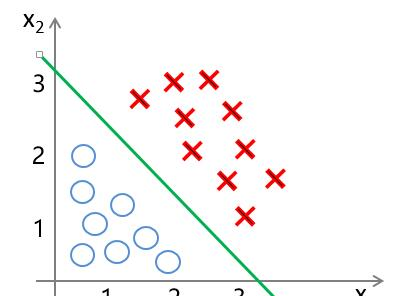
使用邏輯回歸進行分類，就是要找到綠色這樣的分界線，使其能夠盡可能地對樣本進行正确分類，也就是能夠盡可能地将兩種樣本分隔開來。是以我們可以構造這樣一個函數，來對樣本集進行分隔：

z ( x ( i ) ) = θ 0 + θ 1 x 1 ( i ) + θ 2 x 2 ( i ) + . . . + θ n x n ( i ) z(x^{(i)}) = \theta_0 + \theta_1 x^{(i)}_1 + \theta_2 x^{(i)}_2 + ... + \theta_n x^{(i)}_n z(x(i))=θ0​+θ1​x1(i)​+θ2​x2(i)​+...+θn​xn(i)​

其中 i=1,2,…m，表示第 i個樣本, n 表示特征數,當 z ( x ( i ) ) > 0 z(x^{(i)}) > 0 z(x(i))>0 時，對應着樣本點位于分界線上方，可将其分為"1"類；當 z ( x ( i ) ) < 0 z(x^{(i)}) < 0 z(x(i))<0 時 ，樣本點位于分界線下方，将其分為“0”類。

邏輯回歸作為分類算法，它的輸出是0/1。那麼如何将輸出值轉換成0/1呢？

這就需要一個新的函數——sigmoid 函數

sigmoid 函數

sigmoid 函數定義如下：

g ( z ) = 1 1 + e − z g(z) = \frac{1}{1+e^{-z}} g(z)=1+e−z1​

其函數圖像為：

由函數圖像可以看出， sigmoid函數可以很好地将 (−∞,∞) 内的數映射到 (0,1) 上。

是以我們可以認為g（z）>= 0.5時為“1”類，反之為“0”類

y = { 1 , if  g ( z ) ≥ 0.5   0 , otherwise y = \begin{cases} 1, & \text {if $g(z) \geq 0.5$ } \\ 0, & \text{otherwise} \end{cases} y={1,0,​if g(z)≥0.5 otherwise​

二項邏輯斯蒂回歸模型(binomial logistic regression model)是一種分類模型，由條件機率分布 p(Y|X)表示，形式為參數化的邏輯斯谛分布。這裡，随機變量 X 取值為實數，随機變量 Y 取值為 1或0。可通過監督學習的方法來估計模型參數。

二項邏輯斯谛回歸模型是如下的條件機率分布：

p ( Y = 1 ∣ x ) = e θ T x 1 + e θ T x p(Y=1|x) = \frac{e^{\theta^Tx}}{1+e^{\theta^Tx}} p(Y=1∣x)=1+eθTxeθTx​

p ( Y = 0 ∣ x ) = 1 1 + e θ T x p(Y=0|x) = \frac{1}{1+e^{\theta^Tx}} p(Y=0∣x)=1+eθTx1​

其中， x∈Rn 是輸入， Y∈{0,1} 是輸出， θ 是參數。

對于 Y=1 ：

p ( Y = 1 ∣ x ) = e θ T x 1 + e θ T x p(Y=1|x) = \frac{e^{\theta^Tx}}{1+e^{\theta^Tx}} p(Y=1∣x)=1+eθTxeθTx​

而 e θ T x ≠ 0 e^{\theta^Tx} \neq 0 eθTx​=0,故：

p ( Y = 1 ∣ x ) = 1 1 + e − θ T x p(Y=1|x) = \frac{1}{1+e^{-\theta^Tx}} p(Y=1∣x)=1+e−θTx1​

即邏輯回歸模型函數：

h θ ( x ( i ) ) = 1 1 + e − θ T x ( i ) h_\theta(x^{(i)}) = \frac{1}{1+e^{-\theta^Tx^{(i)}}} hθ​(x(i))=1+e−θTx(i)1​

表示為分類結果為“1”的機率

邏輯回歸函數

分類邊界：

z ( x ( i ) ) = θ 0 + θ 1 x 1 ( i ) + θ 2 x 2 ( i ) = θ T x ( i ) z(x^{(i)}) = \theta_0 + \theta_1 x^{(i)}_1 + \theta_2 x^{(i)}_2 = \theta^T x^{(i)} z(x(i))=θ0​+θ1​x1(i)​+θ2​x2(i)​=θTx(i)

其中，$ \theta =[θ_0 θ_1 θ_2 ⋮ θ_n ]$

$ x^{(i)} = \begin{bmatrix} x^{(i)}_0 \ x^{(i)}_1 \ x^{(i)}_2 \ \vdots \ x^{(i)}_n \ \end{bmatrix} $

  而 x(i)0=1是偏置項, n 表示特征數，i=1,2,…,m 表示樣本數。

sigmoid函數 ：

g ( z ) = 1 1 + e − z g(z) = \frac{1}{1+e^{-z}} g(z)=1+e−z1​

則***邏輯回歸模型函數***為

h θ ( x ( i ) ) = g ( z ) = g ( θ T x ( i ) ) = 1 1 + e − θ T x i h_\theta(x^{(i)}) = g(z) = g( \theta^T x^{(i)} ) = \frac{1}{1+e^{-\theta^T x^{i}}} hθ​(x(i))=g(z)=g(θTx(i))=1+e−θTxi1​

我們可以對于新樣本 $ x^{new} = [x^{new}1, x{new}*2,…,x{new}n]^T 進行輸入，得到函數值進行輸入，得到函數值 h\theta(x^{new}) ,根據 h\theta(x^{new}) $ 與0.5的比較來将新樣本進行分類。

代價函數

使用 sigmoid 函數求解出來的值為類1的後驗估計 p(y=1|x,θ),故我們可以得到：

p ( y = 1 ∣ x , θ ) = h θ ( θ T x ) p(y=1|x,\theta) = h_\theta(\theta^T x) p(y=1∣x,θ)=hθ​(θTx)

則

p ( y = 0 ∣ x , θ ) = 1 − h θ ( θ T x ) p(y=0|x,\theta) = 1- h_\theta(\theta^T x) p(y=0∣x,θ)=1−hθ​(θTx)

其中 p(y=1|x,θ)表示樣本分類為 y=1 的機率，而 p(y=0|x,θ) 表示樣本分類為 y=0的機率。針對以上二式，我們可将其整理為：

p ( y ∣ x , θ ) = p ( y = 1 ∣ x , θ ) y p ( y = 0 ∣ x , θ ) ( 1 − y ) = h θ ( θ T x ) y ( 1 − h θ ( θ T x ) ) ( 1 − y ) p(y|x,\theta)=p(y=1|x,\theta)^y p(y=0|x,\theta)^{(1-y)} = h_\theta(\theta^T x)^y (1- h_\theta(\theta^T x))^{(1-y)} p(y∣x,θ)=p(y=1∣x,θ)yp(y=0∣x,θ)(1−y)=hθ​(θTx)y(1−hθ​(θTx))(1−y)

我們可以得到其似然函數為：

L ( θ ) = ∏ i = 1 m p ( y ( i ) ∣ x ( i ) , θ ) = ∏ i = 1 m [ h θ ( θ T x ( i ) ) y ( i ) ( 1 − h θ ( θ T x ( i ) ) ) 1 − y ( i ) ] L(\theta) = \prod^m_{i=1} p(y^{(i)}|x^{(i)},\theta) = \prod ^m_{i=1}[ h_\theta(\theta^T x^{(i)})^{y^{(i)}} (1- h_\theta(\theta^T x^{(i)}))^{1-y^{(i)}}] L(θ)=i=1∏m​p(y(i)∣x(i),θ)=i=1∏m​[hθ​(θTx(i))y(i)(1−hθ​(θTx(i)))1−y(i)]

 對數似然函數為：

log ⁡ L ( θ ) = ∑ i = 1 m [ y ( i ) log ⁡ h θ ( θ T x ( i ) ) + ( 1 − y ( i ) ) log ⁡ ( 1 − h θ ( θ T x ( i ) ) ) ] \log L(\theta) = \sum_{i=1}^m [y^{(i)} \log{h_\theta(\theta^T x^{(i)})} +(1-y^{(i)}) \log{(1- h_\theta(\theta^T x^{(i)}))}] logL(θ)=i=1∑m​[y(i)loghθ​(θTx(i))+(1−y(i))log(1−hθ​(θTx(i)))]

 于是，我們便得到了代價函數，我們可以對求 logL(θ)log⁡L(θ) 的最大值來求得參數 θθ 的值。為了便于計算，将代價函數做了以下改變：

J ( θ ) = − 1 m ∑ i = 1 m [ y ( i ) log ⁡ h θ ( θ T x ( i ) ) + ( 1 − y ( i ) ) log ⁡ ( 1 − h θ ( θ T x ( i ) ) ) ] J(\theta) = - \frac{1}{m} \sum_{i=1}^m [y^{(i)} \log{h_\theta(\theta^T x^{(i)})} + (1-y^{(i)}) \log{(1- h_\theta(\theta^T x^{(i)}))}] J(θ)=−m1​i=1∑m​[y(i)loghθ​(θTx(i))+(1−y(i))log(1−hθ​(θTx(i)))]

 此時，我們隻需對 J(θ)求最小值，便得可以得到參數 θ。

三、優化算法

梯度下降

梯度下降法過程為： θ j : = θ j − α Δ J ( θ ) Δ θ j \theta_j := \theta_j - \alpha \frac{\Delta J(\theta)}{\Delta \theta_j} θj​:=θj​−αΔθj​ΔJ(θ)​

求解梯度:

而

我們又知道：

那麼：

是以有：

綜上：

随機梯度下降法

随機梯度下降是每次疊代使用一個樣本來對參數進行更新。

即

僞代碼：

repeat{

    for i=1,…,m{

       θ j : = θ j − α 1 m ( h θ ( x ( i ) ) − y ( i ) ) x j ( i ) \theta_j := \theta_j -\alpha \frac{1}{m}(h_{\theta}(x^{(i)})-y^{(i)})x_j^{(i)} θj​:=θj​−αm1​(hθ​(x(i))−y(i))xj(i)​

      (for j =0,1)

    }

  }

優點：

  （1）由于不是在全部訓練資料上的損失函數，而是在每輪疊代中，随機優化某一條訓練資料上的損失函數，這樣每一輪參數的更新速度大大加快。

  缺點：

  （1）準确度下降。由于即使在目标函數為強凸函數的情況下，SGD仍舊無法做到線性收斂。

  （2）可能會收斂到局部最優，由于單個樣本并不能代表全體樣本的趨勢。

  （3）不易于并行實作。

牛頓法

牛頓法是一種在實數域和複數域上近似求解方程的方法。方法使用函數f (x)的泰勒級數的前面幾項來尋找方程f (x) = 0的根。牛頓法最大的特點就在于它的收斂速度很快。

步驟：

首先，選擇一個接近函數 f (x)零點的 x0，計算相應的 f (x0) 和切線斜率f ’ (x0)（這裡f ’ 表示函數 f 的導數）。然後我們計算穿過點(x0, f (x0)) 并且斜率為f '(x0)的直線和 x 軸的交點的x坐标，也就是求如下方程的解：

我們将新求得的點的 x 坐标命名為x1，通常x1會比x0更接近方程f (x) = 0的解。是以我們現在可以利用x1開始下一輪疊代。疊代公式可化簡為如下所示：

已經證明，如果f ’ 是連續的，并且待求的零點x是孤立的，那麼在零點x周圍存在一個區域，隻要初始值x0位于這個鄰近區域内，那麼牛頓法必定收斂。 并且，如果f ’ (x)不為0, 那麼牛頓法将具有平方收斂的性能. 粗略的說，這意味着每疊代一次，牛頓法結果的有效數字将增加一倍。下圖為一個牛頓法執行過程的例子。

由于牛頓法是基于目前位置的切線來确定下一次的位置，是以牛頓法又被很形象地稱為是"切線法"。牛頓法的搜尋路徑（二維情況）如下圖所示：

而在邏輯回歸中牛頓法更新方式為：

本質上去看，牛頓法是二階收斂，梯度下降是一階收斂，是以牛頓法就更快。如果更通俗地說的話，比如你想找一條最短的路徑走到一個盆地的最底部，梯度下降法每次隻從你目前所處位置選一個坡度最大的方向走一步，牛頓法在選擇方向時，不僅會考慮坡度是否夠大，還會考慮你走了一步之後，坡度是否會變得更大。是以，可以說牛頓法比梯度下降法看得更遠一點，能更快地走到最底部。（牛頓法目光更加長遠，是以少走彎路；相對而言，梯度下降法隻考慮了局部的最優，沒有全局思想。）

紅色的牛頓法的疊代路徑，綠色的是梯度下降法的疊代路徑。

優點：二階收斂，收斂速度快；

缺點：牛頓法是一種疊代算法，每一步都需要求解目标函數的Hessian矩陣的逆矩陣，計算比較複雜。Hessian矩陣也存在不可逆的情況

拟牛頓法

牛頓法中的Hesse矩陣H在稠密時求逆計算量大，也有可能沒有逆（Hesse矩陣非正定）。拟牛頓法提出，用不含二階導數的矩陣 Ut 替代牛頓法中的 Ht−1，然後沿搜尋方向 −Utgt 做一維搜尋。根據不同的 Ut 構造方法有不同的拟牛頓法。

拟牛頓條件

牛頓法的搜尋方向是 d ( t ) = − H t − 1 g t d^{(t)}=-H_t^{-1}g_t d(t)=−Ht−1​gt​

為了不算二階導及其逆矩陣，設法構造一個矩陣 U，用它來逼近 H−1

現在為了友善推導，假設 f(x) 是二次函數，于是 Hesse 矩陣 H 是常數陣，任意兩點 x(t)和 x(t+1)處的梯度之差是：

▽ f ( x ( t + 1 ) ) − ▽ f ( x ( t ) ) = H ⋅ ( x ( t + 1 ) − x ( t ) ) \bigtriangledown f(x^{(t+1)}) - \bigtriangledown f(x^{(t)}) = H\cdot (x^{(t+1)}-x^{(t)}) ▽f(x(t+1))−▽f(x(t))=H⋅(x(t+1)−x(t))

等價于

x ( t + 1 ) − x ( t ) = H − 1 ⋅ [ ▽ f ( x ( t + 1 ) ) − ▽ f ( x ( t ) ) ] x^{(t+1)}-x^{(t)} = H^{-1}\cdot [\bigtriangledown f(x^{(t+1)}) - \bigtriangledown f(x^{(t)})] x(t+1)−x(t)=H−1⋅[▽f(x(t+1))−▽f(x(t))]

那麼對非二次型的情況，也仿照這種形式，要求近似矩陣 U 滿足類似的關系：

x ( t + 1 ) − x ( t ) = U t + 1 ⋅ [ ▽ f ( x ( t + 1 ) ) − ▽ f ( x ( t ) ) ] x^{(t+1)}-x^{(t)}=U_{t+1}\cdot [\bigtriangledown f(x^{(t+1)})-\bigtriangledown f(x^{(t)})] x(t+1)−x(t)=Ut+1​⋅[▽f(x(t+1))−▽f(x(t))]

或者寫成

Δ x t = U t + 1 ⋅ Δ g t \Delta x_t=U_{t+1}\cdot \Delta g_t Δxt​=Ut+1​⋅Δgt​

BFGS算法是最流行的拟牛頓算法。

BFGS算法（Broyden-Fletcher-Goldfarb-Shanno）

自适應梯度算法(Adagrad)

在實際應用中，各參數的重要性肯定是不同的，是以對于不同的參數要進行動态調整，采取不同的學習率，讓目标函數能夠更快地收斂。

将每一個參數的每一次疊代的梯度取平方，然後累加并開方得到 r，最後用全局學習率除以 r，作為學習率的動态更新。

令 α 表示全局學習率，r 為梯度累積變量，初始值為 0。

1. 單獨計算每一個參數在目前位置的梯度。

g = ∂ L ( w ) ∂ w i g=\frac{∂L(w)}{∂w_i} g=∂wi​∂L(w)​

1. 累積平方梯度，一般來說 g 是一個向量，而向量的平方通常寫為 gTg

   r = r + g 2 或 r = r + g T g r=r+g^2 或r=r+g^Tg r=r+g2或r=r+gTg

2. 更新參數

w = w − α r g w=w-\frac{\alpha}{\sqrt{r}}g w=w−r

​α​g

上述式子存在一個問題，r 在計算過程中有可能變為 0，在代碼中分母為零通常都會報錯，是以我們需要想辦法讓分母不為零，同時不會影響到參數的更新。

我們可以在分母上加一個極小的常數 σ，因為取值極小，即使開方後仍然不會影響參數的更新。通常，σ 大約設定為 10 的 -7 次方。

w = w − α σ + r g w=w-\frac{\alpha}{\sigma+\sqrt{r}}g w=w−σ+r

​α​g

AdaDelta算法

Adadelta是對Adagrad的擴充，最初方案依然是對學習率進行自适應限制，但是進行了計算上的簡化。

特點：

• 訓練國中期，加速效果不錯，很快
• 訓練後期，反複在局部最小值附近抖動

RMSProp

因為Adagrad算法會出現提前停止的現象，是以在RMSProp算法中解決了這個問題，它采用指數權重平均的思想，隻将最近的梯度進行累加計算平方。

s t = γ s t − 1 + ( 1 − γ ) ▽ θ J ( θ ) ∗ ▽ θ J ( θ ) s_{t} = \gamma s_{t-1} + (1 - \gamma)\bigtriangledown_\theta J(\theta) * \bigtriangledown_\theta J(\theta) st​=γst−1​+(1−γ)▽θ​J(θ)∗▽θ​J(θ)

θ = θ − η s t + ϵ ∗ ▽ θ J ( θ ) \theta = \theta - \frac{\eta}{\sqrt{s_{t} + \epsilon}} * \bigtriangledown_\theta J(\theta) θ=θ−st​+ϵ

​η​∗▽θ​J(θ)

Adam

Adam算法和傳統的随機梯度下降不同。随機梯度下降保持單一的學習率（即alpha）更新所有的權重，學習率在訓練過程中并不會改變。而Adam通過随機梯度的一階矩估計和二階矩估計而為不同的參數設計獨立的自适應性學習率。

四、代碼實作

導入包

import math
import csv
import numpy as np
           

讀取資料

def loaddata(filename):
    label = []
    with open(filename, 'r') as f:
        lines = csv.reader(f)
        data = list(lines)
    for i in range(len(data)):
        del(data[i][0])
        for j in range(len(data[i])):
            data[i][j] = float(data[i][j])
        label.append(data[i][-1])
        del(data[i][-1])
    return np.array(data), np.array(label)
           

代價函數

def J(theta, X, Y, theLambda=0):
    m, n = X.shape
    h = sigmoid(np.dot(X, theta))
    J = (-1.0/m)*(np.dot(np.log(h).T, Y)+np.dot(np.log(1-h).T, 1-Y)) + (theLambda/(2.0*m))*np.sum(np.square(theta[1:]))

    return J.flatten()[0]
           

sigmod函數

def sigmoid(x):
    return 1.0/(1 + np.exp(-x))
           

随機梯度下降

def gradient_sgd(X, Y, alpha=0.01, epsilon=0.00001, maxloop=1000, theLambda=0.0):

    m, n = X.shape

    theta = np.zeros((n, 1))

    cost = J(theta, X, Y)
    costs = [cost]
    thetas = [theta]

    # 随機梯度下降
    count = 0
    flag = False
    while count < maxloop:
        if flag:
            break

        for i in range(m):
            h = sigmoid(np.dot(X[i].reshape((1, n)), theta))

            theta = theta - alpha * (
                        (1.0 / m) * X[i].reshape((n, 1)) * (h - Y[i]) + (theLambda / m) * np.r_[[[0]], theta[1:]])
            thetas.append(theta)
            cost = J(theta, X, Y, theLambda)
            costs.append(cost)
            if abs(costs[-1] - costs[-2]) < epsilon:
                flag = True
                break
        count += 1

        if count % 100 == 0:
            print("cost:", cost)

    return thetas, costs, count
           

牛頓法

def gradient_newton(X, Y, epsilon=0.00001, maxloop=1000, theLambda=0.0):

    m, n = X.shape

    theta = np.zeros((n, 1))

    cost = J(theta, X, Y)
    costs = [cost]
    thetas = [theta]

    count = 0

    while count < maxloop:

        delta_J = 0.0
        H = 0.0

        for i in range(m):
            h = sigmoid(np.dot(X[i].reshape((1, n)), theta))

            delta_J += X[i] * (h - Y[i])

            H += h.T * (1 - h) * X[i] * X[i].T


        delta_J /= m
        H /= m

        print(H, delta_J)

        theta = theta - 1.0 / H * delta_J

        thetas.append(theta)
        cost = J(theta, X, Y, theLambda)
        costs.append(cost)

        if abs(costs[-1] - costs[-2]) < epsilon:
            break
        count += 1

        if count % 100 == 0:
            print("cost:", cost)

    return thetas, costs, count
           

Adagrad

def gradient_adagrad(X, Y, alpha=0.01, sigma=1e-7, epsilon=0.00001, maxloop=1000, theLambda=0.0):

    m, n = X.shape

    theta = np.zeros((n, 1))

    r = [[0.0] for _ in range(n)]


    cost = J(theta, X, Y)
    costs = [cost]
    thetas = [theta]

    count = 0
    flag = False
    while count < maxloop:
        if flag:
            break

        for i in range(m):
            h = sigmoid(np.dot(X[i].reshape((1, n)), theta))

            grad = (1.0 / m) * X[i].reshape((n, 1)) * (h - Y[i])

            for j in range(n):
                r[j].append(grad[j]**2+r[j][-1])
                theta[j] = theta[j] - alpha * grad[j] / (sigma + math.sqrt(r[j][-1]))

            thetas.append(theta)
            cost = J(theta, X, Y, theLambda)
            costs.append(cost)
            if abs(costs[-1] - costs[-2]) < epsilon:
                flag = True
                break
        count += 1

        if count % 100 == 0:
            print("cost:", cost)
    return thetas, costs, count
           

Adadelta

def gradient_adadelta(X, Y, rho=0.01, alpha=0.01, sigma=1e-7, epsilon=0.00001, maxloop=1000, theLambda=0.0):

    m, n = X.shape

    theta = np.zeros((n, 1))

    r = [[0.0] for _ in range(n)]
    deltax = [[0.0] for _ in range(n)]
    deltax_ = [[1.0] for _ in range(n)]


    cost = J(theta, X, Y)
    costs = [cost]
    thetas = [theta]

    count = 0
    flag = False
    while count < maxloop:
        if flag:
            break

        for i in range(m):
            h = sigmoid(np.dot(X[i].reshape((1, n)), theta))

            grad = (1.0 / m) * X[i].reshape((n, 1)) * (h - Y[i])

            for j in range(n):
                r[j].append((1-rho) * grad[j]**2 + rho * r[j][-1])

                deltax[j].append(- (math.sqrt(deltax_[j][-1] / sigma + r[j][-1]))*alpha)

                theta[j] = theta[j] + deltax[j][-1]

                deltax_[j].append((1-rho)*deltax[j][-1]**2+rho*deltax_[j][-1])
                # print(deltax)
                # print(deltax_)

            thetas.append(theta)
            cost = J(theta, X, Y, theLambda)
            costs.append(cost)
            if abs(costs[-1] - costs[-2]) < epsilon:
                flag = True
                break
        count += 1

        if count % 100 == 0:
            print("cost:", cost)

    return thetas, costs, count
           

RMSProp

def gradient_RMSProp(X, Y, rho=0.01, alpha=0.01, sigma=1e-7, epsilon=0.00001, maxloop=1000, theLambda=0.0):

    m, n = X.shape

    theta = np.zeros((n, 1))

    r = [[0.0] for _ in range(n)]


    cost = J(theta, X, Y)
    costs = [cost]
    thetas = [theta]

    count = 0
    flag = False
    while count < maxloop:
        if flag:
            break

        for i in range(m):
            h = sigmoid(np.dot(X[i].reshape((1, n)), theta))

            grad = (1.0 / m) * X[i].reshape((n, 1)) * (h - Y[i])

            for j in range(n):
                r[j].append((1 - rho)*grad[j]**2+rho*r[j][-1])
                theta[j] = theta[j] - alpha * grad[j] / (sigma + math.sqrt(r[j][-1]))

            thetas.append(theta)
            cost = J(theta, X, Y, theLambda)
            costs.append(cost)
            if abs(costs[-1] - costs[-2]) < epsilon:
                print(costs)
                flag = True
                break
        count += 1

        if count % 100 == 0:
            print("cost:", cost)
    return thetas, costs, count
           

Adam

def gradient_adam(X, Y, rho1=0.9, rho2=0.999, alpha=0.01, sigma=1e-7, epsilon=0.00001, maxloop=1000, theLambda=0.0):

    m, n = X.shape

    theta = np.zeros((n, 1))

    s = [[0.0] for _ in range(n)]
    r = [[0.0] for _ in range(n)]

    cost = J(theta, X, Y)
    costs = [cost]
    thetas = [theta]

    count = 0
    flag = False
    while count < maxloop:
        if flag:
            break

        for i in range(m):
            h = sigmoid(np.dot(X[i].reshape((1, n)), theta))

            grad = (1.0 / m) * X[i].reshape((n, 1)) * (h - Y[i])

            for j in range(n):
                r[j].append((1 - rho2)*grad[j]**2+rho2*r[j][-1])
                s[j].append((1 - rho1)*grad[j]+rho1*r[j][-1])

                theta[j] = theta[j] - alpha * (s[j][-1]/(1-rho1**2))/(math.sqrt(r[j][-1]/(1-rho2**2))+sigma)

            thetas.append(theta)
            cost = J(theta, X, Y, theLambda)
            costs.append(cost)
            if abs(costs[-1] - costs[-2]) < epsilon:
                print(costs)
                flag = True
                break
        count += 1

        if count % 100 == 0:
            print("cost:", cost)
    return thetas, costs, count
           

主程式

if __name__ == '__main__':
    train_data, train_label = loaddata('data/data43561/pima_train.csv')
    test_data, test_label = loaddata('data/data43561/pima_test.csv')

    # print(train_data)
    # print(train_label)

    m = train_data.shape[0]
    # print(m)
    X = np.concatenate((np.ones((m, 1)), train_data), axis=1)
    # print(X)

    thetas, costs, iterationCount = gradient_sgd(X, train_label, 0.05, 0.00000001, 100)
    # thetas, costs, iterationCount = gradient_newton(X, train_label, 0.00000001, 10000)
    # thetas, costs, iterationCount = gradient_adagrad(X, train_label, 0.05, 1e-7, 0.000000000000001, 10000)
    # thetas, costs, iterationCount = gradient_adadelta(X, train_label, 0.9999999999, 1e-5, 1e-7, 0.000000000000001, 10000)
    # thetas, costs, iterationCount = gradient_RMSProp(X, train_label, 0.9, 1e-5, 1e-7, 0.000000000000001, 10000)
    # thetas, costs, iterationCount = gradient_adam(X, train_label, 0.9, 0.99, 0.001, 1e-7, 0.000000000000001, 10000)
    print(costs[-1], iterationCount)
           

/opt/conda/envs/python35-paddle120-env/lib/python3.7/site-packages/ipykernel_launcher.py:4: RuntimeWarning: divide by zero encountered in log
  after removing the cwd from sys.path.
/opt/conda/envs/python35-paddle120-env/lib/python3.7/site-packages/ipykernel_launcher.py:26: RuntimeWarning: invalid value encountered in double_scalars


cost: 0.7724120224525658
0.7724120224525658 100
           

運作代碼請點選：https://aistudio.baidu.com/aistudio/projectdetail/625618?shared=1