Hisat2/StringTie/Ballgown轉錄組資料分析執行個體（拟南芥）

RNA-Seq for Model Plant (Arabidopsis thaliana)

參考文章

https://bi.biopapyrus.jp/rnaseq/mapping/hista/hisat2-paired-rnaseq.html

下載下傳資料

直接利用參考文章裡的shell腳本

SEQLIBS=(SRR8428909 SRR8428908 SRR8428907 SRR8428906 SRR8428905 SRR8428904)

for seqlib in ${SEQLIBS[@]}; do
    wget ftp://ftp.sra.ebi.ac.uk/vol1/fastq/SRR842/00${seqlib:9:10}/${seqlib}/${seqlib}_1.fastq.gz
    wget ftp://ftp.sra.ebi.ac.uk/vol1/fastq/SRR842/00${seqlib:9:10}/${seqlib}/${seqlib}_2.fastq.gz
done

複制

執行

bash download_raw_data.sh

複制

資料對應的文章

https://www.ncbi.nlm.nih.gov/pubmed?LinkName=sra_pubmed&from_uid=7072798

基本的實驗設計：野生型對應轉基因株系

解壓重命名

bgzip -d SRR8428909_1.fastq.gz
bgzip -d SRR8428909_2.fastq.gz

mv SRR8428909_1.fastq wt_Rep1_R1.fastq
mv SRR8428909_2.fastq wt_Rep1_R2.fastq

bgzip -d SRR8428908_1.fastq.gz
bgzip -d SRR8428908_2.fastq.gz

mv SRR8428908_1.fastq wt_Rep2_R1.fastq
mv SRR8428908_2.fastq wt_Rep2_R2.fastq

bgzip -d SRR8428907_1.fastq.gz
bgzip -d SRR8428907_2.fastq.gz

mv SRR8428907_1.fastq wt_Rep3_R1.fastq
mv SRR8428907_2.fastq wt_Rep3_R2.fastq

bgzip -d SRR8428906_1.fastq.gz
bgzip -d SRR8428906_2.fastq.gz

mv SRR8428906_1.fastq EE_Rep1_R1.fastq
mv SRR8428906_2.fastq EE_Rep1_R2.fastq

bgzip -d SRR8428905_1.fastq.gz
bgzip -d SRR8428905_2.fastq.gz

mv SRR8428905_1.fastq EE_Rep2_R1.fastq
mv SRR8428905_2.fastq EE_Rep2_R2.fastq

bgzip -d SRR8428904_1.fastq.gz
bgzip -d SRR8428904_2.fastq.gz

mv SRR8428904_1.fastq EE_Rep3_R1.fastq
mv SRR8428904_2.fastq EE_Rep3_R2.fastq

複制

在windows電腦上寫到shell腳本在linux運作的時候遇到報錯

2_unzip_raw_data.sh: line 3: $'\r': command not found

修改一下

sed -i 's/\r$//' 2_unzip_raw_data.sh

複制

使用fastp對資料進行過濾

SEQLIBS=(EE_Rep1 EE_Rep2 EE_Rep3 wt_Rep1 wt_Rep2 wt_Rep3)

for seqlib in ${SEQLIBS[@]}; do
    fastp -i ${seqlib}_R1.fastq -I ${seqlib}_R2.fastq -o ${seqlib}_clean_R1.fastq -O ${seqlib}_clean_R2.fastq
done

複制

下載下傳參考基因組和注釋檔案

wget ftp://ftp.ensemblgenomes.org/pub/plants/release-40/fasta/arabidopsis_thaliana/dna/Arabidopsis_thaliana.TAIR10.dna.toplevel.fa.gz
bgzip -d Arabidopsis_thaliana.TAIR10.dna.toplevel.fa.gz
wget ftp://ftp.ensemblgenomes.org/pub/plants/release-40/gff3/arabidopsis_thaliana/Arabidopsis_thaliana.TAIR10.40.gff3.gz
bgzip -d Arabidopsis_thaliana.TAIR10.40.gff3.gz

複制

hisat2建構索引

mkdir reference
mv Arabidopsis_thaliana* reference
cd reference
hisat2-build Arabidopsis_thaliana.TAIR10.dna.toplevel.fa tair10

複制

hisat2比對

SEQLIBS=(EE_Rep1 EE_Rep2 EE_Rep3 wt_Rep1 wt_Rep2 wt_Rep3)

for seqlib in ${SEQLIBS[@]}; do
    hisat2 -x reference/tair10 -1 ${seqlib}_clean_R1.fastq -2 ${seqlib}_clean_R2.fastq -p 4 -S ${seqlib}.sam
done

複制

sam檔案轉換為bam檔案并排序

SEQLIBS=(EE_Rep1 EE_Rep2 EE_Rep3 wt_Rep1 wt_Rep2 wt_Rep3)

for seqlib in ${SEQLIBS[@]}; do
    samtools view -@ 8 -bhS ${seqlib}.sam -o ${seqlib}.bam
	samtools sort -@ 8 ${seqlib}.bam -o ${seqlib}.sorted.bam
done

複制

把之前下載下傳的gff3檔案轉化為gtf格式

cd reference
gffread Arabidopsis_thaliana.TAIR10.40.gff3 -o TAIR10_GFF3_genes.gtf

複制

接下來的具體步驟我也暫時看不明白具體是做啥了，反正最後得到的就是ballgown的輸入檔案了

stringtie -p 8 -l wT1 -G reference/TAIR10_GFF3_genes.gtf -o athaliana_wt_Rep1/transcripts.gtf wt_Rep1.sorted.bam
stringtie -p 8 -l wT2 -G reference/TAIR10_GFF3_genes.gtf -o athaliana_wt_Rep2/transcripts.gtf wt_Rep2.sorted.bam
stringtie -p 8 -l wT3 -G reference/TAIR10_GFF3_genes.gtf -o athaliana_wt_Rep3/transcripts.gtf wt_Rep3.sorted.bam

stringtie -p 8 -l EE1 -G reference/TAIR10_GFF3_genes.gtf -o athaliana_EE_Rep1/transcripts.gtf EE_Rep1.sorted.bam
stringtie -p 8 -l EE2 -G reference/TAIR10_GFF3_genes.gtf -o athaliana_EE_Rep2/transcripts.gtf EE_Rep2.sorted.bam
stringtie -p 8 -l EE3 -G reference/TAIR10_GFF3_genes.gtf -o athaliana_EE_Rep3/transcripts.gtf EE_Rep3.sorted.bam

ls -l athaliana_*/*.gtf | awk '{print $9}' > sample_assembly_gtf_list.txt

stringtie --merge -p 8 -o stringtie_merged.gtf -G reference/TAIR10_GFF3_genes.gtf sample_assembly_gtf_list.txt
gffcompare -r reference/TAIR10_GFF3_genes.gtf -o gffcompare stringtie_merged.gtf
stringtie -e -B -p 4 wt_Rep1.sorted.bam -G stringtie_merged.gtf -o athaliana_wt_Rep1/athaliana_wt_Rep1
stringtie -e -B -p 4 wt_Rep2.sorted.bam -G stringtie_merged.gtf -o athaliana_wt_Rep2/athaliana_wt_Rep2.count -A athaliana_wt_Rep2/wt_Rep2_gene_abun.out
stringtie -e -B -p 4 wt_Rep3.sorted.bam -G stringtie_merged.gtf -o athaliana_wt_Rep3/athaliana_wt_Rep3.count -A athaliana_wt_Rep3/wt_Rep3_gene_abun.out
stringtie -e -B -p 4 EE_Rep1.sorted.bam -G stringtie_merged.gtf -o athaliana_EE_Rep1/athaliana_EE_Rep1.count -A athaliana_EE_Rep1/EE_Rep1_gene_abun.out
stringtie -e -B -p 4 EE_Rep2.sorted.bam -G stringtie_merged.gtf -o athaliana_EE_Rep2/athaliana_EE_Rep2.count -A athaliana_EE_Rep2/EE_Rep2_gene_abun.out
stringtie -e -B -p 4 EE_Rep3.sorted.bam -G stringtie_merged.gtf -o athaliana_EE_Rep3/athaliana_EE_Rep3.count -A athaliana_EE_Rep3/EE_Rep3_gene_abun.out

複制

将以下檔案導出到本地，放到一個檔案夾下，我放到了ballgown這個檔案夾下

[1] "athaliana_EE_Rep1" "athaliana_EE_Rep2" "athaliana_EE_Rep3" [4] "athaliana_wt_Rep1" "athaliana_wt_Rep2" "athaliana_wt_Rep3"

接下來開始差異表達分析

list.files("ballgown/")
sample<-c("athaliana_EE_Rep1","athaliana_EE_Rep2", "athaliana_EE_Rep3", "athaliana_wt_Rep1", "athaliana_wt_Rep2", "athaliana_wt_Rep3" )
type<-c(rep("EE",3),rep("wt",3))
pheno_df<-data.frame("sample"=sample,"type"=type)
rownames(pheno_df)<-pheno_df[,1]
pheno_df
BiocManager::install("ballgown")
library(ballgown)
BiocManager::install("alyssafrazee/RSkittleBrewer")
library(RSkittleBrewer)
library(genefilter)
library(dplyr)
library(ggplot2)
library(gplots)
library(devtools)
install.packages("RFLPtools")
library(RFLPtools)
bg <- ballgown(dataDir = "./ballgown/", pData=pheno_df, samplePattern = "athaliana")
gene_expression<-gexpr(bg)
head(gene_expression)
boxplot(log10(gene_expression+1),names=c("EE1","EE2","EE3","WT1","WT2","WT3"),
        col=c("red", "red","red","blue", "blue","blue"))

複制

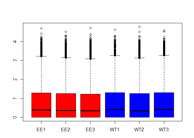
Hisat2/StringTie/Ballgown轉錄組資料分析執行個體（拟南芥）

image.png

samples<-c("EE1","EE2","EE3","WT1","WT2","WT3")
colnames(gene_expression)<-samples
rv<-rowVars(gene_expression)
select<-order(rv,decreasing = T)[seq_len(min(500,length(rv)))]
pc<-prcomp(t(gene_expression[select,]),scale=T)
pc$x
scores<-data.frame(pc$x,samples)
scores
pcpcnt<-round(100*pc$sdev^2/sum(pc$sdev^2),1)
names(pcpcnt)<-paste0("PC",1:6)
pcpcnt
point_colors<-c(rep("red",3),rep("blue",3))
plot(pc$x[,1],pc$x[,2], xlab="", ylab="", main="PCA plot for all libraries",xlim=c(min(pc$x[,1])-2,max(pc$x[,1])+2),ylim=c(min(pc$x[,2])-2,max(pc$x[,2])+2),col=point_colors)
text(pc$x[,1],pc$x[,2],pos=2,rownames(pc$x), col=c("red", "red","red","blue", "blue", "blue"))

複制

image.png

results_transcripts<-stattest(bg,feature="transcript",covariate = 'type',
                              getFC=T,meas="FPKM")
results_genes<-stattest(bg,feature="gene",covariate="type",getFC=T,meas="FPKM")
results_genes["log2fc"]<-log2(results_genes$fc)
head(results_genes)
g_sign<-subset(results_genes,pval<0.1&abs(log2fc)>0.584)
head(g_sign)
dim(g_sign)
write.csv(g_sign,"results_genes.csv",row.names=F,quote = F)
DEG<-results_genes
DEG$change<-as.factor(ifelse(DEG$pval<0.05&abs(DEG$log2fc)>0.5,
                             ifelse(DEG$log2fc>0.5,"UP","DOWN"),
                             "NOT"))
DEG<-na.omit(DEG)
ggplot(data=DEG,aes(x=log2fc,y=-log10(pval),color=change))+
  geom_point(alpha=0.4,size=1.75)+
  labs(x="log2 fold change")+ ylab("-log10 pvalue")+
  theme_bw(base_size = 20)+
  theme(plot.title = element_text(size=15,hjust=0.5))+
  scale_color_manual(values=c('blue','black','red'))

複制

image.png

接下來還有GO注釋和網絡分析的内容，另外找時間來做了

簡單總結

能夠運作完基本流程，但是stringtie做了啥，ballgown做了啥，還有對應的參數是什麼意思暫時還不太清楚，還的話時間看這兩個軟體！