Node Measures and Computation in Social Media Analysis

Node Measures and Computation

1.Node Centrality

1. Geometric Centrality Measures

• (In)Degree Centrality

The Number of incoming links

C

d

e

f

(

x

)

=

d

i

n

(

x

)

C_{def}(x) = d_{in}(x)

Cdef​(x)=din​(x)

Equivalently to the number of nodes at distance one or to the majority voting.

• Closeness Centrality

Nodes that are more central have smaller distances

C

c

l

o

s

(

c

)

=

1

∑

d

(

y

,

x

)

C_{}clos(c) = \frac{1}{\sum d{(y,x)}}

C​clos(c)=∑d(y,x)1​

d

(

y

,

x

)

d(y,x)

d(y,x) is the length of ther shortest path from y to x

Nodes that are more central have smaller distances to other nodes and higher centrality.

The graph must be (strongly) connected!

• In the mathematical theory of directed graphs, a graph is said to be strongly connected if every vertex is reachable from every other vertex. The strongly connected components of an arbitrary directed graph form a partition into subgraphs that are themselves strongly connected. It is possible to test the strong connectivity of a graph, or to find its strongly connected components, in linear time (that is, Θ(V+E)).
• In graph theory, a component, sometimes called a connected component, of an undirected graph is a subgraph in which any two vertices are connected to each other by paths, and which is connected to no additional vertices in the supergraph.

• Harmonic Centrality

C

h

a

r

(

x

)

=

∑

y

≠

x

1

d

(

y

,

x

)

=

∑

d

(

y

,

x

)

<

∞

,

y

≠

x

1

d

(

y

,

x

)

C_{har}(x) = \sum_{y \neq x} \frac{1}{d(y,x)} = \sum_{d(y,x) < \infin , y \neq x} \frac{1}{d(y,x)}

Char​(x)=y​=x∑​d(y,x)1​=d(y,x)<∞,y​=x∑​d(y,x)1​

• Strongly correalted to closeness centrality
• Naturally aslo accounts for nodes y that cannot reach x
• Can be applied to graphs that are Note Strongly Connected

Harmonic Centrality can be normalized by dividing by N-1, where N is the number of nodes in the graph:

C

c

h

a

r

(

x

)

=

1

n

−

1

∑

y

≠

x

1

d

(

y

,

x

)

=

1

n

−

1

∑

d

(

y

,

x

)

<

∞

,

y

≠

x

1

d

(

y

,

x

)

C_{char}(x) = \frac{1}{n-1} \sum_{y \neq x} \frac{1}{d(y,x)} = \frac{1}{n-1} \sum_{d(y,x) < \infin , y \neq x} \frac{1}{d(y,x)}

Cchar​(x)=n−11​y​=x∑​d(y,x)1​=n−11​d(y,x)<∞,y​=x∑​d(y,x)1​

2. Spectral Centrality Measures

• Eigenvevtor Centrality

In degree centrality, we consider nodes with more connections to be more important. However, in real-world scenarios, having more friends does not by itself guarantee that someone is important: having more important friends provides a stronger signal.

Eigenvector centrality tries to generalize degree centrality by incorporat- ing the importance of the neighbors (or incoming neighbors in directed graphs). It is defined for both directed and undirected graphs. To keep track of neighbors, we can use the adjacency matrix A of a graph.

• We assume the eigenvector centrality of a node is

  C

  e

  (

  V

  i

  )

  C_e(V_i)

  Ce​(Vi​)

• We would like

  C

  e

  (

  V

  i

  )

  C_e(V_i)

  Ce​(Vi​) to be higher when important neighbors point to in.

  - for incoming neighbors

  A

  j

  ,

  i

  =

  1

  A_{j,i} = 1

  Aj,i​=1

• Each node starts with the same score, and then each node gives away its score to its successors, and then normai

  C

  e

  (

  V

  i

  )

  =

  1

  λ

  ∑

  j

  =

  1

  n

  A

  j

  ,

  i

  C

  e

  (

  V

  j

  )

  C_e(V_i) = \frac{1}{\lambda} \sum_{j=1}^{n} A_{j,i}C_e(V_j)

  Ce​(Vi​)=λ1​j=1∑n​Aj,i​Ce​(Vj​)

$\lambda $

is the norm of the centrality vector of all nodes.

Let

C

e

=

(

C

e

(

V

1

)

,

C

e

(

V

2

)

,

…

,

C

e

(

V

n

)

)

T

C_e = (C_e(V_1),C_e(V_2), \dots , C_e(V_n))^T

Ce​=(Ce​(V1​),Ce​(V2​),…,Ce​(Vn​))T

$ \lambda C_e = A^T C_e $

This means that

C

e

C_{e}

Ce​`is an eigenvector of adjacency matrix

A

T

A_T

AT​and

λ

\lambda

λ is the corresponding eigenvalue.

We should choose the largest eigenvalue and the corresponding eigenvector. And the lagrest value in this vector is the most central node.

For example, here’s an undirected graph:

So this is the adjacency matrix:

Let’s calculate the eigenvector and eigenvalue by Matlab:

We can find that the 2.6855 is the largest eigenvalue so we normalize the corresponding eigenvector and find the second value is the largest. So node

V

2

V_2

V2​ is the most central nodes.

• Katz Centrality

A major problem with eigen vector centrality arise when it deals with directed graphs. For nodes without incoming edges in a directed graph, their centrality valurs are zero. Eigenvector centrality only considers the effect of network topology structure and cannot capture the external knowledge. To resolve this problem we add bias term

$\beta$

to the centrality values for all nodes:

C

K

a

t

z

(

V

i

)

=

α

∑

j

=

1

n

A

j

,

i

C

K

a

t

z

(

V

j

)

+

β

C_{Katz}(V_i) = \alpha \sum_{j=1}^n A_{j,i}C_{Katz}(V_j)+\beta

CKatz​(Vi​)=αj=1∑n​Aj,i​CKatz​(Vj​)+β

Katz Centrality:

C

K

a

t

z

=

β

(

I

−

α

A

T

)

−

1

⋅

1

C_{Katz} = \beta (I - \alpha A^T) ^ {-1} · 1

CKatz​=β(I−αAT)−1⋅1

$\alpha < \frac{1}{ \lambda }` is selected so that the matrix is inertible.

Let’s take this graph for example:

The adjacency matrix is

A = 
\begin{bmatrix}
 0 &1  &1  &1  &0 \\ 
 1 &0  &1  &1  &1 \\ 
 1 &1  &0  &1  &1 \\ 
 1 &1  &1  &0  &0 \\ 
 0 &1  &1  &0  &0 
\end{bmatrix} = A^T
           

The Eigenvalues are -1.68, -1.0, -1.0, 0.35, 3.32.

We assume

$\alpha < 1/3.32$

and

$\beta$

= 0.2

C_{Katz} = \beta (I-\alpha A^T)^{-1}·1 = 
\begin{bmatrix}
1.14\\ 
1.31\\ 
1.31\\ 
1.14\\ 
0.85
\end{bmatrix}
           

So the node

$V_2$

and node

$V_3$

are the most important nodes.

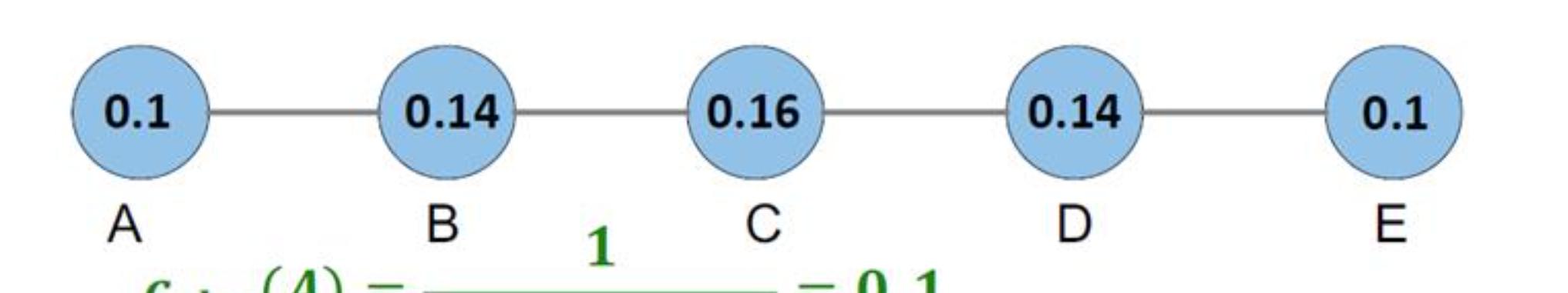
• PageRank

In directed graphs, once a ndoe becomes an authortity(high centrality), it passes all its centrality along all of its out-links. This is less desirable since not everyone known by a well-known person is well-knows.

So we can divide the value of passed centrality by the number of outgoing links. Each connected neighbor gets a fraction of the source node’s centrality.

C_p = \beta (I - \alpha A^TD^{-1})^{-1} · 1
           

This is similar to Katz Centrality,

$ \alpha < 1 / \lambda $

,where

$\lambda$

is the largest eigenvalue of

$A^TD^{-1}$

. In undirected graphs, the largest eigenvalue of

$A^TD^{-1}$

. In undirected graphs, the largest eigenvalue of

$AA^TD^{-1}$

is

$\lambda = 1$

; therefore ,

$\alpha < 1$

.

$\beta$

is often set as

$1-\alpha$

.

And D is the degree matrix.

$D = [d_{ii}], d_{ii}$

is the degree of node i. For example in this graph:

The degree matrix is

\begin{bmatrix}
3 &0  &0  & 0 & 0 & 0\\ 
0&  2&  0&  0&  0& 0\\ 
 0&  0&  3& 0 & 0 & 0\\ 
0 & 0 & 0 &  3&  0&0 \\ 
0 &0  & 0 & 0 &  0&0 \\ 
0 &  0& 0 &  0&  0& 2
\end{bmatrix}
           

The inverse of matrix D will also be a diagonal n x n matrix in the floowing form:

\begin{bmatrix}
\frac{1}{d_1} &0  &\dots& 0\\ 
0&  \frac{1}{d_2}&  0&  0\\ 
\vdots&  0&  \ddots& \vdots \\ 
0 & 0 & \dots &\frac{1}{d_n} \\
\end{bmatrix}
           

When the out-degree is zero, in this situation, the

$A_{j,i} = 0$

. This makes the term inside the summation

$\frac{0}{0}$

. We can fix this problem by setting

$d_{j}^{out} = 1$

since the node will not contribute any centrality to any other nodes.

Here is a PageRank example:

A = 
\begin{bmatrix}
 0 &1  &0  &1  &1 \\ 
 1 &0  &1  &0  &1 \\ 
 0 &1  &0  &1  &1 \\ 
 1 &0  &1  &0  &0 \\ 
 1 &1  &1  &0  &0 
\end{bmatrix}
           

D = 
\begin{bmatrix}
 3 &0  &0  &0  &0\\ 
 0 &3  &0  &0  &0\\ 
 0 &0  &3  &0  &0\\ 
 0 &0  &0  &2  &0 \\ 
 0 &0  &0  &0  &3
\end{bmatrix}
           

C_p = \beta (I - \alpha A^TD^{-1})^{-1} ·1 = 
\begin{bmatrix}
2.14\\
2.13\\
2.14\\
1.45\\
2.13
\end{bmatrix}
           

So the node

$V_1$

and

$V_3$

are most important.

• Hits Centrality

In a directed graph, a node is more important if it has more link.

Each node has 2 scores:

• Quality as an expert(hub樞紐): Total sum of votes(authority scores) of nodes that it points to
• Quality as a content provider(autority權重): Total sum of votes(hub scores) from nodes that point to it

Authorities are nodes containing useful information, for instance the newspaper home page the search engine home page etc.

Hubs are nodes that link to autorities, for example Hao123.com

When we counting in-links authority. Each hub page startes with hub score 1 authorities collect their votes. And hubs collect authority. And authorities collect hub scores again.

• A good hub links to mang good authorities

• A good authority is linked from many good hubs.

  We can use the former two properities and based on the mutual reinforcement method to do iteration. Each iteration will update these two values, until they stop changing.

C_{aut}(x) = \sum _{y\rightarrow x}c_{hub}(y)
           

C_{hub}(c) = \sum _{x\rightarrow y}c_{aut}(y) 
           

++HIts algorithm:++

Each page i has 2 scores:

• Authority score:

  $a_i$

• Hub score:

  $h_i$

  Convergence criteria:

\sum _{i}(h_i^{(t)}-h_i^{(t+1)})^2 < \epsilon
           

\sum _{i}(a_i^{(t)}-a_i^{(t+1)})^2 < \epsilon
           

• Initialize:

  $a^{(0)}_j = 1/ \sqrt n$

  ,

  $h_j^{(0)} = 1/\sqrt n$

• Theen keep iterating until conveergence:

\forall i: Autority: a_i^{(t+1)} = \sum _{j\rightarrow i} h_j^{(t)}
           

\forall i: Hub: h_i^{(t+1)} = \sum _{j\rightarrow i} a_j^{(t)}
           

\forall i: Normalize: a_i^{(t+1)} = a_i^{(t+1)}/\sqrt{\sum_i (a_i ^{(T+1)})^2} 
           

h_i^{(t+1)} = h_i^{(t+1)}/\sqrt{\sum_i (h_i ^{(T+1)})^2}
           

• Hits in the vector notation:
• vector

  $a = (a_1 \dots , a_n), h = (h_1 \dots, h_n)$

• Adjacency matrix A(n x n):

  $A_{ij} = 1$

  if

  $i \rightarrow j$

• Can rewrite

  $h_i = \sum_{i \rightarrow j} a_j$

  as

  $h_i = \sum_{j} A_{ij}·a_j$

• So: h = A·a and simlilarly:

  $a = A^T·h$

• Repeat until convergence:

• $h(t+1) = A·a(t)$

• $a^(t+1) = A^T·h^{(t)}$

• Normalize

  $a^{(t+1)}$

  and

  $h^{(t+1)}$

The steady state (HITS has converged) is:

a = A^T ·(A·a)/c^`
           

A^T·A·a = c^` · a
           

A·A^T ·h = c^{``} · h
           

So, authority a is eigenveotor of

$A^T A$

(associated with the largest eigenvalue) Similarly: hub h is eigenvector of

$AA^T$

.

The shortage of HITs

1. 計算效率較低

   因為HITS算法是與查詢相關的算法，是以必須在接收到使用者查詢後實時進行計算，而HITS算法本身需要進行很多輪疊代計算才能獲得最終結果，這導緻其計算效率較低，這是實際應用時必須慎重考慮的問題。

2. 主題飄移問題

   如果在擴充網頁集合裡包含部分與查詢主題無關的頁面，而且這些頁面之間有較多的互相連結指向，那麼使用HITS算法很可能會給予這些無關網頁很高的排名，導緻搜尋結果發生主題漂移，這種現象被稱為“緊密連結社群現象”（Tightly-Knit CommunityEffect）。

3. 易被作弊者操縱結果

   HITS從機制上很容易被作弊者操縱，比如作弊者可以建立一個網頁，頁面内容增加很多指向高品質網頁或者著名網站的網址，這就是一個很好的Hub頁面，之後作弊者再将這個網頁連結指向作弊網頁，于是可以提升作弊網頁的Authority得分。

4. 結構不穩定

   所謂結構不穩定，就是說在原有的“擴充網頁集合”内，如果添加删除個别網頁或者改變少數連結關系，則HITS算法的排名結果就會有非常大的改變。

• The difference between HITS and PageRank

HITS算法和PageRank算法可以說是搜尋引擎連結分析的兩個最基礎且最重要的算法。從以上對兩個算法的介紹可以看出，兩者無論是在基本概念模型還是計算思路以及技術實作細節都有很大的不同，下面對兩者之間的差異進行逐一說明.

1.HITS算法是與使用者輸入的查詢請求密切相關的，而PageRank與查詢請求無關。是以，HITS算法可以單獨作為相似性計算評價标準，而PageRank必須結合内容相似性計算才可以用來對網頁相關性進行評價；

2.HITS算法因為與使用者查詢密切相關，是以必須在接收到使用者查詢後實時進行計算，計算效率較低；而PageRank則可以在爬蟲抓取完成後離線計算，線上直接使用計算結果，計算效率較高；

3.HITS算法的計算對象數量較少，隻需計算擴充集合内網頁之間的連結關系；而PageRank是全局性算法，對所有網際網路頁面節點進行處理；

4.從兩者的計算效率和處理對象集合大小來比較，PageRank更适合部署在伺服器端，而HITS算法更适合部署在用戶端；

5.HITS算法存在主題泛化問題，是以更适合處理具體化的使用者查詢；而PageRank在處理寬泛的使用者查詢時更有優勢；

6.HITS算法在計算時，對于每個頁面需要計算兩個分值，而PageRank隻需計算一個分值即可；在搜尋引擎領域，更重視HITS算法計算出的Authority權值，但是在很多應用HITS算法的其它領域，Hub分值也有很重要的作用；

7.從連結反作弊的角度來說，PageRank從機制上優于HITS算法，而HITS算法更易遭受連結作弊的影響。

8.HITS算法結構不穩定，當對“擴充網頁集合”内連結關系作出很小改變，則對最終排名有很大影響；而PageRank相對HITS而言表現穩定，其根本原因在于PageRank計算時的“遠端跳轉”

• Power Iteration Method

There is also a power iteration method to compute the eigen-centrality, Katz centrality and PageRank.

• Eigen-centrality:

• Set

  $C^{(0)} \leftarrow 1, k \leftarrow 1 $

• 1:

  $C^{(k)} \leftarrow A^TC^{(k-1)}$

• 2.

  $C^{(k)} = c^{(k)}/ \left \| c^{(k)} \right \|_2 \rightarrow \lambda$

• 3.if

  $ \left \| C^{(k)} - C^{(k-1)} \right \| > \epsilon$

  :
• 4.

  $k \leftarrow k+1$

  , goto step 1

  

• Katz Centrality

• Set

  $C^{(0)} \leftarrow 1, k \leftarrow 1 $

• 1:

  $C^{(k)} \leftarrow \alpha A^TC^{(k-1)} + \beta _1$

• 2.if

  $ \left \| C^{(k)} - C^{(k-1)} \right \| > \epsilon$

  :
• 3.

  $k \leftarrow k+1$

  , goto step 1

• PageRank

Referring to the power iteration algorithm for Katz Centrality. Just replace the adjacency matrix by

$A^TD^{-1}$

.

3.Path-based Measures of Centrality

• Edge Betweenness

Number of shortest paths passing over the edge

Step to compute edge betweenness

• Forward step: Count the number of shortest paths

  $\sigma_{ai} $

  from A to all other nodes i of the network.
• Backwared step: Compute betweenness: If there are multiple paths count them fractionally

• Node betweenness Centrality

Another way of loking at centrality is by considering how important nodes are in connecting other nodes.

C_b(V_i) = \sum _{s \neq t\neq V_i} \frac{\sigma_{st} (V_i)}{\sigma_{st}}
           

$\sigma_{st}$

The number of shortest paths from vertex s to t - a.k.a. information pathways

$\sigma_{st} (V_i)$

The number of ++shortest path++ from s to t that pass through

$V_i$

• betweenness centrality example1:

  

• betweenness centrality example2:

  

• Brandes Algorithm

A better way to compute the node betweenness

C_b(V_i) = \sum _{s \neq t\neq V_i} \frac{\sigma_{st} (V_i)}{\sigma_{st}} = \sum_{s \neq V_i} \delta_s (V_i)
           

\delta_s(V_i) = \sum_{t \neq V_i} \frac{\sigma_{st}(V_i)}{\sigma_{st}}
           

$\delta_s(V_i)$

- the dependence of s to

$V_i$

There exist a recurrence equation that can help us determine

$\sigma_s(V_i)$

\delta_s(V_i) = \sum_{w:V_i \in pred(s,w)} \frac{\sigma_{SV_I}}{\sigma_{sw}} (1+\sigma_s(w))
           

pred(s,w) is the set of predecessors of w in the shortest paths from s to w.

-

$V_i$

is one of parents nodes of w

- if w is not

$V_i$

's child node, it can be ignored.

3.Node Similarity Computation

• Structural equivalence

- We look at the neighborhood shared by two nodes

- The size of this shared neighborhood defines how similar two nodes are.

• Vertex Similarity

\sigma(v_i,v_j) = |N(v_i) \cap N(v_j)|
           

• Jaccard Similarity

\sigma_{jaccard}(v_i,v_j) = \frac{|N(v_i) \cap N(v_j)|}{|N(v_i) \cup N(v_j)|}
           

• Cosine Similarity

\sigma_{Cosine}(v_i,v_j) = \frac{|N(v_i) \cap N(v_j)|}{\sqrt {|N(v_i) || N(v_j)|}}
           

And here is a example of computer the similarity:

However, we often excludes the node itself in the neighborhood. In this situation, some connected nodes not sharing a neighbor will be assigned zero similarity. For example, there are two nodes a and b, they are connnected without any neighbors. If we exclude them then they doesn’t have any neighbor, and those similarity value will be zero.

So, in the above case, when we include them into calculation. The result will become as followed:

\sigma_{Jaccard}(v_2,v_5) = \frac{|[v_1,v_2,v_3,v_4] \cap [v_3,v_5,v_6]|}{|[v_1,v_2,v_3,v_4,v_5,v_6]|} = \frac{1}{6}
           

\sigma_{Cosine}(v_2,v_5) = \frac{|[v_1,v_2,v_3,v_4] \cap [v_3,v_5,v_6]|}{\sqrt{[v_1,v_2,v_3,v_4] || [v_3,v_5,v_6]}} = \frac{1}{\sqrt {12}} = 0.29