用機器學習來預測天氣Part 1

概述

  本章是使用機器學習預測天氣系列教程的第一部分，使用Python和機器學習來構模組化型，根據從Weather Underground收集的資料來預測天氣溫度。該教程将由三個不同的部分組成，涵蓋的主題是：

• 資料收集和處理（本文）
• 線性回歸模型（第2章）
• 神經網絡模型（第3章）

  本教程中使用的資料将從Weather Underground的免費層API服務中收集。我将使用python的requests庫來調用API，得到從2015年起Lincoln, Nebraska的天氣資料。 一旦收集完成，資料将需要進行處理并彙總轉成合适的格式，然後進行清理。   第二篇文章将重點分析資料中的趨勢，目标是選擇合适的特性并使用python的statsmodels和scikit-learn庫來建構線性回歸模型。 我将讨論建構線性回歸模型，必須進行必要的假設，并示範如何評估資料特征以建構一個健壯的模型。 并在最後完成模型的測試與驗證。   最後的文章将着重于使用神經網絡。 我将比較建構神經網絡模型和建構線性回歸模型的過程，結果，準确性。

Weather Underground介紹

  Weather Underground是一家收集和分發全球各種天氣測量資料的公司。 該公司提供了大量的API，可用于商業和非商業用途。 在本文中，我将介紹如何使用非商業API擷取每日天氣資料。是以，如果你跟随者本教程操作的話，您需要注冊他們的免費開發者帳戶。 此帳戶提供了一個API密鑰，這個密鑰限制，每分鐘10個，每天500個API請求。   擷取曆史資料的API如下：

http://api.wunderground.com/api/API_KEY/history_YYYYMMDD/q/STATE/CITY.json             

複制

• API_KEY: 注冊賬戶擷取
• YYYYMMDD: 你想要擷取的天氣資料的日期
• STATE: 州名縮寫
• CITY: 你請求的城市名

調用API

  本教程調用Weather Underground API擷取曆史資料時，用到如下的python庫。

名稱	描述	來源
datetime	處理日期	标準庫
time	處理時間	标準庫
collections	使用該庫的namedtuples來結構化資料	标準庫
pandas	處理資料	第三方
requests	HTTP請求處理庫	第三方
matplotlib	制圖庫	第三方

  好，我們先導入這些庫：

from datetime import datetime, timedelta  
import time  
from collections import namedtuple  
import pandas as pd  
import requests  
import matplotlib.pyplot as plt             

複制

接下裡，定義常量來儲存API_KEY和BASE_URL，注意，例子中的API_KEY不可用，你要自己注冊擷取。代碼如下：

API_KEY = '7052ad35e3c73564'  
# 第一個大括号是API_KEY，第二個是日期
BASE_URL = "http://api.wunderground.com/api/{}/history_{}/q/NE/Lincoln.json"             

複制

然後我們初始化一個變量，存儲日期，然後定義一個list，指明要從API傳回的内容裡擷取的資料。然後定義一個namedtuple類型的變量DailySummary來存儲傳回的資料。代碼如下：

target_date = datetime(2016, 5, 16)  
features = ["date", "meantempm", "meandewptm", "meanpressurem", "maxhumidity", "minhumidity", "maxtempm",  
            "mintempm", "maxdewptm", "mindewptm", "maxpressurem", "minpressurem", "precipm"]
DailySummary = namedtuple("DailySummary", features)             

複制

定義一個函數，調用API，擷取指定target_date開始的days天的資料，代碼如下：

def extract_weather_data(url, api_key, target_date, days):  
    records = []
    for _ in range(days):
        request = BASE_URL.format(API_KEY, target_date.strftime('%Y%m%d'))
        response = requests.get(request)
        if response.status_code == 200:
            data = response.json()['history']['dailysummary'][0]
            records.append(DailySummary(
                date=target_date,
                meantempm=data['meantempm'],
                meandewptm=data['meandewptm'],
                meanpressurem=data['meanpressurem'],
                maxhumidity=data['maxhumidity'],
                minhumidity=data['minhumidity'],
                maxtempm=data['maxtempm'],
                mintempm=data['mintempm'],
                maxdewptm=data['maxdewptm'],
                mindewptm=data['mindewptm'],
                maxpressurem=data['maxpressurem'],
                minpressurem=data['minpressurem'],
                precipm=data['precipm']))
        time.sleep(6)
        target_date += timedelta(days=1)
    return records           

複制

首先，定義個list records，用來存放上述的DailySummary，使用for循環來周遊指定的所有日期。然後生成url，發起HTTP請求，擷取傳回的資料，使用傳回的資料，初始化DailySummary，最後存放到records裡。通過這個函數的出，就可以擷取到指定日期開始的N天的曆史天氣資料，并傳回。

擷取500天的天氣資料

  由于API接口的限制，我們需要兩天的時間才能擷取到500天的資料。你也可以下載下傳我的測試資料，來節約你的時間。

records = extract_weather_data(BASE_URL, API_KEY, target_date, 500)             

複制

格式化資料為Pandas DataFrame格式

  我們使用DailySummary清單來初始化Pandas DataFrame。DataFrame資料類型是機器學習領域經常會用到的資料結構。

df = pd.DataFrame(records, columns=features).set_index('date')           

複制

特征提取

  機器學習是帶有實驗性質的，是以，你可能遇到一些沖突的資料或者行為。是以，你需要在你用機器學習處理問題是，你需要對處理的問題領域有一定的了解，這樣可以更好的提取資料特征。   我将采用如下的資料字段，并且，使用過去三天的資料作為預測。

• mean temperature
• mean dewpoint
• mean pressure
• max humidity
• min humidity
• max dewpoint
• min dewpoint
• max pressure
• min pressure
• precipitation

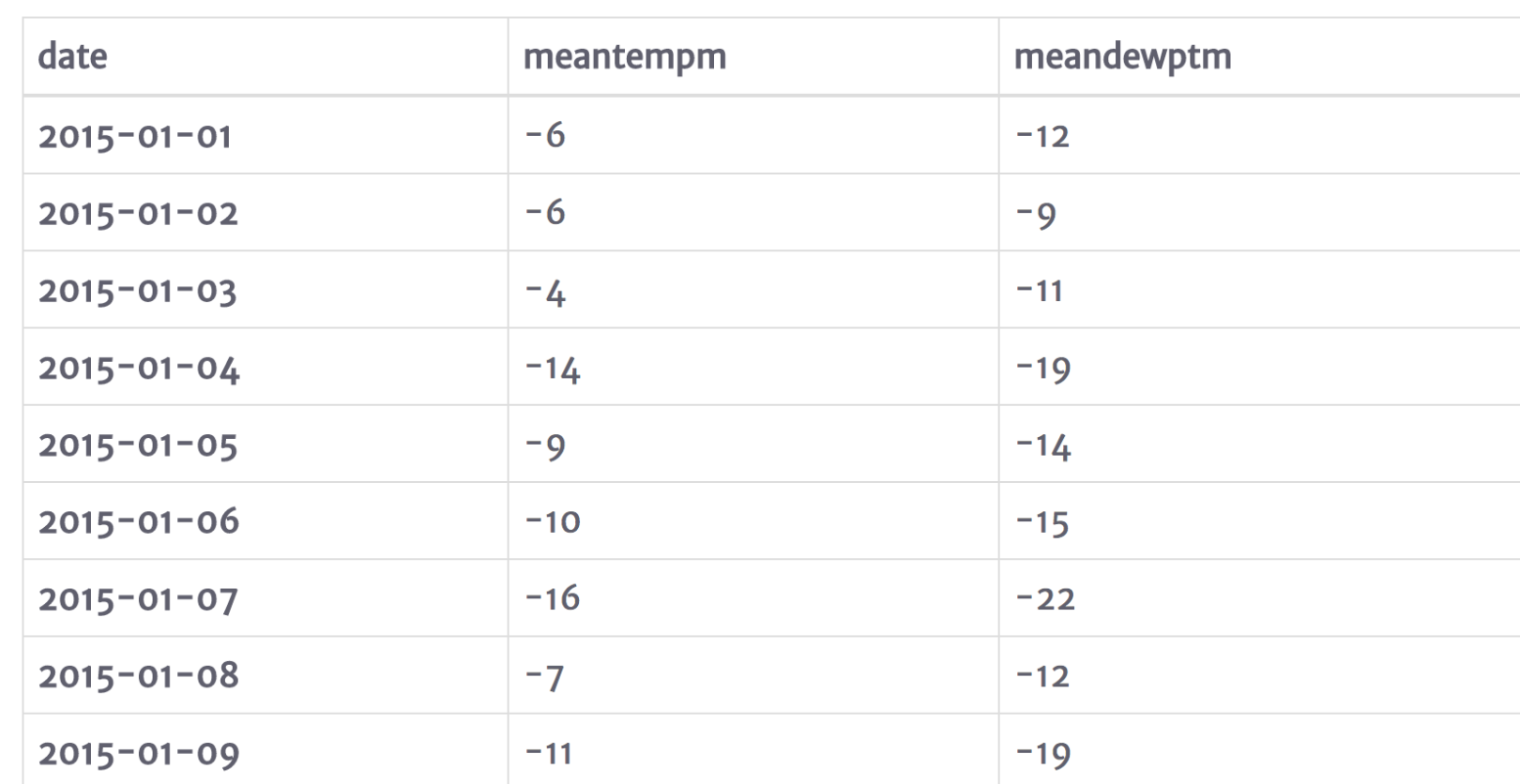
首先我需要在DataFrame裡增加一些字段來儲存新的資料字段，為了友善測試，我建立了一個tmp變量，存儲10個資料，這些資料都有meantempm和meandewptm屬性。代碼如下：

tmp = df[['meantempm', 'meandewptm']].head(10)  
tmp             

複制

對于每一行的資料，我們分别擷取他前一天、前兩天、前三天對應的資料，存在本行，分别以屬性_index來命名，代碼如下：

# 1 day prior
N = 1

# target measurement of mean temperature
feature = 'meantempm'

# total number of rows
rows = tmp.shape[0]

# a list representing Nth prior measurements of feature
# notice that the front of the list needs to be padded with N
# None values to maintain the constistent rows length for each N
nth_prior_measurements = [None]*N + [tmp[feature][i-N] for i in range(N, rows)]

# make a new column name of feature_N and add to DataFrame
col_name = "{}_{}".format(feature, N)  
tmp[col_name] = nth_prior_measurements  
tmp             

複制

我們現在把上面的處理過程封裝成一個函數，友善調用。

def derive_nth_day_feature(df, feature, N):  
    rows = df.shape[0]
    nth_prior_measurements = [None]*N + [df[feature][i-N] for i in range(N, rows)]
    col_name = "{}_{}".format(feature, N)
    df[col_name] = nth_prior_measurements           

複制

好，我們現在對所有的特征，都取過去三天的資料，放在本行。

for feature in features:  
    if feature != 'date':
        for N in range(1, 4):
            derive_nth_day_feature(df, feature, N)           

複制

處理完後，我們現在的所有資料特征為：

df.columns  

Index(['meantempm', 'meandewptm', 'meanpressurem', 'maxhumidity',  
       'minhumidity', 'maxtempm', 'mintempm', 'maxdewptm', 'mindewptm',
       'maxpressurem', 'minpressurem', 'precipm', 'meantempm_1', 'meantempm_2',
       'meantempm_3', 'meandewptm_1', 'meandewptm_2', 'meandewptm_3',
       'meanpressurem_1', 'meanpressurem_2', 'meanpressurem_3',
       'maxhumidity_1', 'maxhumidity_2', 'maxhumidity_3', 'minhumidity_1',
       'minhumidity_2', 'minhumidity_3', 'maxtempm_1', 'maxtempm_2',
       'maxtempm_3', 'mintempm_1', 'mintempm_2', 'mintempm_3', 'maxdewptm_1',
       'maxdewptm_2', 'maxdewptm_3', 'mindewptm_1', 'mindewptm_2',
       'mindewptm_3', 'maxpressurem_1', 'maxpressurem_2', 'maxpressurem_3',
       'minpressurem_1', 'minpressurem_2', 'minpressurem_3', 'precipm_1',
       'precipm_2', 'precipm_3'],
      dtype='object')           

複制

資料清洗

  資料清洗時機器學習過程中最重要的一步，而且非常的耗時、費力。本教程中，我們會去掉不需要的樣本、資料不完整的樣本，檢視資料的一緻性等。   首先去掉我不感興趣的資料，來減少樣本集。我們的目标是根據過去三天的天氣資料預測天氣溫度，是以我們隻保留min, max, mean三個字段的資料。

# make list of original features without meantempm, mintempm, and maxtempm
to_remove = [feature  
             for feature in features 
             if feature not in ['meantempm', 'mintempm', 'maxtempm']]

# make a list of columns to keep
to_keep = [col for col in df.columns if col not in to_remove]

# select only the columns in to_keep and assign to df
df = df[to_keep]  
df.columns
Index(['meantempm', 'maxtempm', 'mintempm', 'meantempm_1', 'meantempm_2',  
       'meantempm_3', 'meandewptm_1', 'meandewptm_2', 'meandewptm_3',
       'meanpressurem_1', 'meanpressurem_2', 'meanpressurem_3',
       'maxhumidity_1', 'maxhumidity_2', 'maxhumidity_3', 'minhumidity_1',
       'minhumidity_2', 'minhumidity_3', 'maxtempm_1', 'maxtempm_2',
       'maxtempm_3', 'mintempm_1', 'mintempm_2', 'mintempm_3', 'maxdewptm_1',
       'maxdewptm_2', 'maxdewptm_3', 'mindewptm_1', 'mindewptm_2',
       'mindewptm_3', 'maxpressurem_1', 'maxpressurem_2', 'maxpressurem_3',
       'minpressurem_1', 'minpressurem_2', 'minpressurem_3', 'precipm_1',
       'precipm_2', 'precipm_3'],
      dtype='object')           

複制

為了更好的觀察資料，我們使用Pandas的一些内置函數來檢視資料資訊，首先我們使用info()函數，這個函數會輸出DataFrame裡存放的資料資訊。

df.info()
<class 'pandas.core.frame.DataFrame'>  
DatetimeIndex: 1000 entries, 2015-01-01 to 2017-09-27  
Data columns (total 39 columns):  
meantempm          1000 non-null object  
maxtempm           1000 non-null object  
mintempm           1000 non-null object  
meantempm_1        999 non-null object  
meantempm_2        998 non-null object  
meantempm_3        997 non-null object  
meandewptm_1       999 non-null object  
meandewptm_2       998 non-null object  
meandewptm_3       997 non-null object  
meanpressurem_1    999 non-null object  
meanpressurem_2    998 non-null object  
meanpressurem_3    997 non-null object  
maxhumidity_1      999 non-null object  
maxhumidity_2      998 non-null object  
maxhumidity_3      997 non-null object  
minhumidity_1      999 non-null object  
minhumidity_2      998 non-null object  
minhumidity_3      997 non-null object  
maxtempm_1         999 non-null object  
maxtempm_2         998 non-null object  
maxtempm_3         997 non-null object  
mintempm_1         999 non-null object  
mintempm_2         998 non-null object  
mintempm_3         997 non-null object  
maxdewptm_1        999 non-null object  
maxdewptm_2        998 non-null object  
maxdewptm_3        997 non-null object  
mindewptm_1        999 non-null object  
mindewptm_2        998 non-null object  
mindewptm_3        997 non-null object  
maxpressurem_1     999 non-null object  
maxpressurem_2     998 non-null object  
maxpressurem_3     997 non-null object  
minpressurem_1     999 non-null object  
minpressurem_2     998 non-null object  
minpressurem_3     997 non-null object  
precipm_1          999 non-null object  
precipm_2          998 non-null object  
precipm_3          997 non-null object  
dtypes: object(39)  
memory usage: 312.5+ KB           

複制

注意：每一行的資料類型都是object，我們需要把資料轉成float。

df = df.apply(pd.to_numeric, errors='coerce')  
df.info()
<class 'pandas.core.frame.DataFrame'>  
DatetimeIndex: 1000 entries, 2015-01-01 to 2017-09-27  
Data columns (total 39 columns):  
meantempm          1000 non-null int64  
maxtempm           1000 non-null int64  
mintempm           1000 non-null int64  
meantempm_1        999 non-null float64  
meantempm_2        998 non-null float64  
meantempm_3        997 non-null float64  
meandewptm_1       999 non-null float64  
meandewptm_2       998 non-null float64  
meandewptm_3       997 non-null float64  
meanpressurem_1    999 non-null float64  
meanpressurem_2    998 non-null float64  
meanpressurem_3    997 non-null float64  
maxhumidity_1      999 non-null float64  
maxhumidity_2      998 non-null float64  
maxhumidity_3      997 non-null float64  
minhumidity_1      999 non-null float64  
minhumidity_2      998 non-null float64  
minhumidity_3      997 non-null float64  
maxtempm_1         999 non-null float64  
maxtempm_2         998 non-null float64  
maxtempm_3         997 non-null float64  
mintempm_1         999 non-null float64  
mintempm_2         998 non-null float64  
mintempm_3         997 non-null float64  
maxdewptm_1        999 non-null float64  
maxdewptm_2        998 non-null float64  
maxdewptm_3        997 non-null float64  
mindewptm_1        999 non-null float64  
mindewptm_2        998 non-null float64  
mindewptm_3        997 non-null float64  
maxpressurem_1     999 non-null float64  
maxpressurem_2     998 non-null float64  
maxpressurem_3     997 non-null float64  
minpressurem_1     999 non-null float64  
minpressurem_2     998 non-null float64  
minpressurem_3     997 non-null float64  
precipm_1          889 non-null float64  
precipm_2          889 non-null float64  
precipm_3          888 non-null float64  
dtypes: float64(36), int64(3)  
memory usage: 312.5 KB             

複制

現在得到我想要的資料了。接下來我們調用describe()函數，這個函數會傳回一個DataFrame，這個傳回值包含了總數、平均數、标準差、最小、25%、50%、75%、最大的資料資訊。

  接下來，使用四分位的方法，去掉25%資料裡特别小的和75%資料裡特别大的資料。

# Call describe on df and transpose it due to the large number of columns
spread = df.describe().T

# precalculate interquartile range for ease of use in next calculation
IQR = spread['75%'] - spread['25%']

# create an outliers column which is either 3 IQRs below the first quartile or
# 3 IQRs above the third quartile
spread['outliers'] = (spread['min']<(spread['25%']-(3*IQR)))|(spread['max'] > (spread['75%']+3*IQR))

# just display the features containing extreme outliers
spread.ix[spread.outliers,]             

複制

  評估異常值的潛在影響是任何分析項目的難點。 一方面，您需要關注引入虛假資料樣本的可能性，這些樣本将嚴重影響您的模型。 另一方面，異常值對于預測在特殊情況下出現的結果是非常有意義的。 我們将讨論每一個包含特征的異常值，看看我們是否能夠得出合理的結論來處理它們。

  第一組特征看起來與最大濕度有關。 觀察這些資料，我可以看出，這個特征類别的異常值是非常低的最小值。這資料看起來沒價值，我想我想仔細看看它，最好是以圖形方式。 要做到這一點，我會使用直方圖。

%matplotlib inline
plt.rcParams['figure.figsize'] = [14, 8]  
df.maxhumidity_1.hist()  
plt.title('Distribution of maxhumidity_1')  
plt.xlabel('maxhumidity_1')  
plt.show()           

複制

檢視maxhumidity字段的直方圖，資料表現出相當多的負偏移。 在選擇預測模型和評估最大濕度影響的強度時，我會牢記這一點。 許多基本的統計方法都假定資料是正态分布的。 現在我們暫時不管它，但是記住這個異常特性。

  接下來我們看另外一個字段的直方圖

df.minpressurem_1.hist()  
plt.title('Distribution of minpressurem_1')  
plt.xlabel('minpressurem_1')  
plt.show()            

複制

  要解決的最後一個資料品質問題是缺失值。 由于我建構DataFrame的時候，缺少的值由NaN表示。 您可能會記得，我通過推導代表前三天測量結果的特征，有意引入了收集資料前三天的缺失值。 直到第三天我們才能開始推導出這些特征，是以很明顯我會想把這些頭三天從資料集中排除出去。 再回頭再看一下上面info()函數輸出的資訊，可以看到包含NaN值的資料特征非常的少，除了我提到的幾個字段，基本就沒有了。因為機器學習需要樣本字段資料的完整性，因為如果我們因為降水量那個字段為空，就去掉樣本，那麼會造成大量的樣本不可用，對于這種情況，我們可以給為空的降水量字段的樣本填入一個值。根據經驗和盡量減少由于填入的值對模型的影響，我決定給為空的降水量字段填入值0。

# iterate over the precip columns
for precip_col in ['precipm_1', 'precipm_2', 'precipm_3']:  
    # create a boolean array of values representing nans
    missing_vals = pd.isnull(df[precip_col])
    df[precip_col][missing_vals] = 0           

複制

填入值後，我們就可以删掉字段值為空的樣本了，隻用調用dropna()函數。

df = df.dropna()             

複制

總結

  這篇文章主要介紹了資料的收集、處理、清洗的流程，本篇文章處理完的處理，将用于下篇文章的模型訓練。   對你來說，這篇文章可能很枯燥，沒啥幹貨，但好的樣本資料，才能訓練處好的模型，是以，樣本資料的收集和處理能力，直接影響你後面的機器學習的效果。