DeepLab-v3(86.9 mIOU)
一、模型
(一)空洞卷積
同v2版本
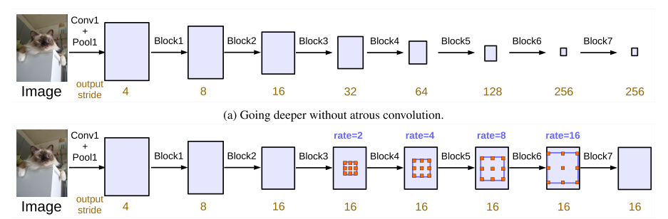
(二)Going deeper
(三)ASPP with BN ( batch normalization )
v3版本的ASPP相對于v2有了一些改進。

如上圖所示,随着rate的變大,有效的卷積區域變得越來越少。在極端情況下,即rate = feature map size時,空洞卷積核的有效卷積區域隻有1。為了解決這一問題,作者對ASPP進行了以下改進:
上圖中黃色括号括起的部分就是改進之後的ASPP,對于輸入的scores map,分别進行五個平行處理:①1×1卷積;②3×3的rate=6的空洞卷積;③3×3的rate=12的空洞卷積;④3×3的rate=18的空洞卷積;⑤全局平均池化+雙線性插值上采樣。五個操作的輸出的尺寸是相同的,對于這五個輸出在通道次元上進行concate;然後再進行1×1的卷積。
下面是得到原圖大小1/16的scores map的例子:
class ASPP(nn.Module):
def __init__(self, num_classes):
super(ASPP, self).__init__()

self.conv_1x1_1 = nn.Conv2d(512, 256, kernel_size=1)
self.bn_conv_1x1_1 = nn.BatchNorm2d(256)

self.conv_3x3_1 = nn.Conv2d(512, 256, kernel_size=3, stride=1, padding=6, dilation=6)
self.bn_conv_3x3_1 = nn.BatchNorm2d(256)

self.conv_3x3_2 = nn.Conv2d(512, 256, kernel_size=3, stride=1, padding=12, dilation=12)
self.bn_conv_3x3_2 = nn.BatchNorm2d(256)

self.conv_3x3_3 = nn.Conv2d(512, 256, kernel_size=3, stride=1, padding=18, dilation=18)
self.bn_conv_3x3_3 = nn.BatchNorm2d(256)

self.avg_pool = nn.AdaptiveAvgPool2d(1)

self.conv_1x1_2 = nn.Conv2d(512, 256, kernel_size=1)
self.bn_conv_1x1_2 = nn.BatchNorm2d(256)

self.conv_1x1_3 = nn.Conv2d(1280, 256, kernel_size=1) # (1280 = 5*256)
self.bn_conv_1x1_3 = nn.BatchNorm2d(256)

self.conv_1x1_4 = nn.Conv2d(256, num_classes, kernel_size=1)

def forward(self, feature_map):
# (feature_map has shape (batch_size, 512, h/16, w/16))

feature_map_h = feature_map.size()[2] # (== h/16)
feature_map_w = feature_map.size()[3] # (== w/16)

out_1x1 = F.relu(self.bn_conv_1x1_1(self.conv_1x1_1(feature_map))) # (shape: (batch_size, 256, h/16, w/16))
out_3x3_1 = F.relu(self.bn_conv_3x3_1(self.conv_3x3_1(feature_map))) # (shape: (batch_size, 256, h/16, w/16))
out_3x3_2 = F.relu(self.bn_conv_3x3_2(self.conv_3x3_2(feature_map))) # (shape: (batch_size, 256, h/16, w/16))
out_3x3_3 = F.relu(self.bn_conv_3x3_3(self.conv_3x3_3(feature_map))) # (shape: (batch_size, 256, h/16, w/16))

out_img = self.avg_pool(feature_map) # (shape: (batch_size, 512, 1, 1))
out_img = F.relu(self.bn_conv_1x1_2(self.conv_1x1_2(out_img))) # (shape: (batch_size, 256, 1, 1))
out_img = F.upsample(out_img, size=(feature_map_h, feature_map_w), mode="bilinear") # (shape: (batch_size, 256, h/16, w/16))

out = torch.cat([out_1x1, out_3x3_1, out_3x3_2, out_3x3_3, out_img], 1) # (shape: (batch_size, 1280, h/16, w/16))
out = F.relu(self.bn_conv_1x1_3(self.conv_1x1_3(out))) # (shape: (batch_size, 256, h/16, w/16))
out = self.conv_1x1_4(out) # (shape: (batch_size, num_classes, h/16, w/16))

return out
經過ASPP之後,再通過上線性插值上采樣恢複到原圖尺寸,就得到了最終的分割圖。在v3中作者沒有對scores map進行CRF處理。
總的模型過程比較簡單,可以分成下面三步:
feature_map = self.resnet(x) # (shape: (batch_size, 512, h/16, w/16))
output = self.aspp(feature_map) # (shape: (batch_size, num_classes, h/16, w/16))
output = F.upsample(output, size=(h, w), mode="bilinear") # (shape: (batch_size, num_classes, h, w))
return output
二、實驗
最高可以達到86.9mIOU