[Reinforcement Learning] Model-Free Control

上篇總結了 Model-Free Predict 問題及方法，本文内容介紹 Model-Free Control 方法，即 "Optimise the value function of an unknown MDP"。

在這裡說明下，Model-Free Predict/Control 不僅适用于 Model-Free 的情況，其同樣适用于 MDP 已知的問題：

• MDP model is unknown, but experience can be sampled.
• MDP model is known, but is too big to use, except by samples.

在正式介紹 Model-Free Control 方法之前，我們先介紹下 On-policy Learning 及 Off-policy Learning。

On-policy Learning vs. Off-policy Learning

On-policy Learning：

• "Learn on the job"
• Learn about policy \(\pi\) from experience sampled from \(\pi\)（即采樣的政策與學習的政策一緻）

Off-policy Learning：

• "Look over someone's shoulder"
• Learn about policy \(\pi\) from experience sampled from \(\mu\)（即采樣的政策與學習的政策不一緻）

On-Policy Monte-Carlo Learning

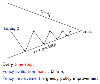
Generalized Policy Iteration

具體的 Control 方法，在《動态規劃》一文中我們提到了 Model-based 下的廣義政策疊代 GPI 架構，那在 Model-Free 情況下是否同樣适用呢？

如下圖為 Model-based 下的廣義政策疊代 GPI 架構，主要分兩部分：政策評估及基于 Greedy 政策的政策提升。


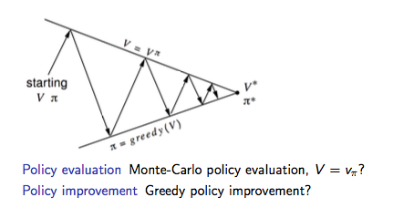
Model-Free 政策評估

在《Model-Free Predict》中我們分别介紹了兩種 Model-Free 的政策評估方法：MC 和 TD。我們先讨論使用 MC 情況下的 Model-Free 政策評估。

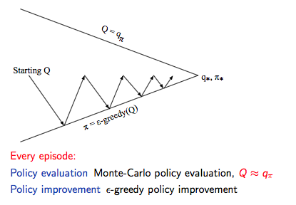
如上圖GPI架構所示：

• 基于 \(V(s)\) 的貪婪政策提升需要 MDP 已知：

\[\pi'(s) = \arg\max_{a\in A}\Bigl(R_{s}^{a}+P_{ss'}^{a}V(s')\Bigr)

\]

• 基于 \(Q(s, a)\) 的貪婪政策提升不需要 MDP 已知，即 Model-Free：

\[\pi'(s) = \arg\max_{a\in A}Q(s, a)

是以 Model-Free 下需要對 \(Q(s, a)\) 政策評估，整個GPI政策疊代也要基于 \(Q(s, a)\)。

Model-Free 政策提升

确定了政策評估的對象，那接下來要考慮的就是如何基于政策評估的結果 \(Q(s, a)\) 進行政策提升。

由于 Model-Free 的政策評估基于對經驗的 samples（即評估的 \(q(s, a)\) 存在 bias），是以我們在這裡不采用純粹的 greedy 政策，防止因為政策評估的偏差導緻整個政策疊代進入局部最優，而是采用具有 explore 功能的 \(\epsilon\)-greedy 算法：

\[\pi(a|s) =

\begin{cases}

&\frac{\epsilon}{m} + 1 - \epsilon, &\text{if } a^*=\arg\max_{a\in A}Q(s, a)\\

&\frac{\epsilon}{m}, &\text{otherwise}

\end{cases}

是以，我們确定了 Model-Free 下的 Monto-Carlo Control：


GLIE

先直接貼下David的課件，GLIE 介紹如下：


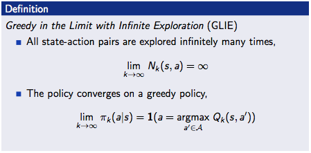
對于 \(\epsilon\)-greedy 算法而言，如果 \(\epsilon\) 随着疊代次數逐漸減為0，那麼 \(\epsilon\)-greedy 是 GLIE，即：

\[\epsilon_{k} = \frac{1}{k}

GLIE Monto-Carlo Control

GLIE Monto-Carlo Control：

• 對于 episode 中的每個狀态 \(S_{t}\) 和動作 \(A_t\)：

\[N(S_t, A_t) ← N(S_t, A_t) + 1 \\

Q(S_t, A_t) ← Q(S_t, A_t) + \frac{1}{N(S_t, A_t)}(G_t - Q(S_t, A_t))

• 基于新的動作價值函數提升政策：

\[\epsilon ← \frac{1}{k}\\

\pi ← \epsilon\text{-greedy}(Q)

定理：GLIE Monto-Carlo Control 收斂到最優的動作價值函數，即：\(Q(s, a) → q_*(s, a)\)。

On-Policy Temporal-Difference Learning

Sarsa

我們之前總結過 TD 相對 MC 的優勢：

• 低方差
• Online
• 非完整序列

那麼一個很自然的想法就是在整個控制閉環中用 TD 代替 MC：

• 使用 TD 來計算 \(Q(S, A)\)
• 仍然使用 \(\epsilon\)-greedy 政策提升
• 每一個 step 進行更新

通過上述改變就使得 On-Policy 的蒙特卡洛方法變成了著名的 Sarsa。

• 更新動作價值函數


- Control


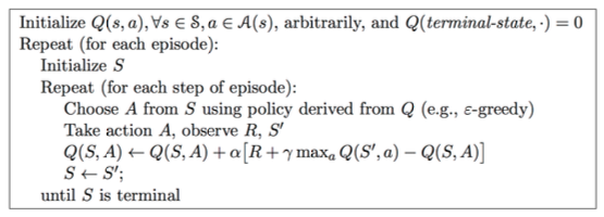
Sarsa算法的僞代碼如下：

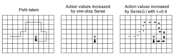
Sarsa(λ)

n-step Sarsa returns 可以表示如下：

\(n=1\) 時：\(q_{t}^{(1)} = R_{t+1} + \gamma Q(S_{t+1})\)

\(n=2\) 時：\(q_{t}^{(2)} = R_{t+1} + \gamma R_{t+2} + \gamma^2 Q(S_{t+2})\)

...

\(n=\infty\) 時：\(q_{t}^{\infty} = R_{t+1} + \gamma R_{t+2} + ... + \gamma^{T-1} R_T\)

是以，n-step return \(q_{t}^{(n)} = R_{t+1} + \gamma R_{t+2} + ... + \gamma^{n}Q(S_{t+n})\)

n-step Sarsa 更新公式：

\[Q(S_t, A_t) ← Q(S_t, A_t) + \alpha (q_t^{(n)} - Q(S_t, A_t))

具體的 Sarsa(λ) 算法僞代碼如下：

其中 \(E(s, a)\) 為資格迹。

下圖為 Sarsa(λ) 用于 Gridworld 例子的示意圖：


Off-Policy Learning

Off-Policy Learning 的特點是評估目标政策 \(\pi(a|s)\) 來計算 \(v_{\pi}(s)\) 或者 \(q_{\pi}(s, a)\)，但是跟随行為政策 \(\{S_1, A_1, R_2, ..., S_T\}\sim\mu(a|s)\)。

Off-Policy Learning 有什麼意義？

• Learn from observing humans or other agents
• Re-use experience generated from old policies \(\pi_1, \pi_2, ..., \pi_{t-1}\)
• Learn about optimal policy while following exploratory policy
• Learn about multiple policies while following one policy

重要性采樣

重要性采樣的目的是：Estimate the expectation of a different distribution。

\[\begin{align}

E_{X\sim P}[f(X)]

&= \sum P(X)f(X)\\

&= \sum Q(X)\frac{P(X)}{Q(X)}f(X)\\

&= E_{X\sim Q}[\frac{P(X)}{Q(X)}f(X)]

\end{align}

Off-Policy MC 重要性采樣

使用政策 \(\pi\) 産生的 return 來評估 \(\mu\)：

\[G_t^{\pi/\mu} = \frac{\pi(A_t|S_t)}{\mu(A_t|S_t)} \frac{\pi(A_{t+1}|S_{t+1})}{\mu(A_{t+1}|S_{t+1})}...\frac{\pi(A_T|S_T)}{\mu(A_T|S_T)}G_t

朝着正确的 return 方向去更新價值：

\[V(S_t) ← V(S_t) + \alpha\Bigl(\color{Red}{G_t^{\pi/\mu}}-V(S_t)\Bigr)

需要注意兩點：

• Cannot use if \(\mu\) is zero when \(\pi\) is non-zero
• 重要性采樣會顯著性地提升方差

Off-Policy TD 重要性采樣

TD 是單步的，是以使用政策 \(\pi\) 産生的 TD targets 來評估 \(\mu\)：

\[V(S_t) ← V(S_t) + \alpha\Bigl(\frac{\pi(A_t|S_t)}{\mu(A_t|S_t)}(R_{t+1}+\gamma V(S_{t+1}))-V(S_t)\Bigr)

• 方差比MC版本的重要性采樣低很多

Q-Learning

前面分别介紹了對價值函數 \(V(s)\) 進行 off-policy 學習，現在我們讨論如何對動作價值函數 \(Q(s, a)\) 進行 off-policy 學習：

• 不需要重要性采樣
• 使用行為政策選出下一步的動作：\(A_{t+1}\sim\mu(·|S_t)\)
• 但是仍需要考慮另一個後繼動作：\(A'\sim\pi(·|S_t)\)
• 朝着另一個後繼動作的價值更新 \(Q(S_t, A_t)\)：

\[Q(S_t, A_t) ← Q(S_t, A_t) + \alpha\Bigl(R_{t+1}+\gamma Q(S_{t+1}, A')-Q(S_t, A_t)\Bigr)

讨論完對動作價值函數的學習，我們接着看如何通過 Q-Learning 進行 Control：

• 行為政策和目标政策均改進
• 目标政策 \(\pi\) 以greedy方式改進：

\[\pi(S_t) = \arg\max_{a'}Q(S_{t+1}, a')

• 行為政策 \(\mu\) 以 \(\epsilon\)-greedy 方式改進
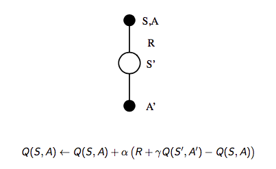
• Q-Learning target：

&R_{t+1}+\gamma Q(S_{t+1}, A')\\

=&R_{t+1}+\gamma Q\Bigl(S_{t+1}, \arg\max_{a'}Q(S_{t+1}, a')\Bigr)\\

=&R_{t+1}+\max_{a'}\gamma Q(S_{t+1}, a')

Q-Learning 的 backup tree 如下所示：


關于 Q-Learning 的結論：

Q-learning control converges to the optimal action-value function, \(Q(s, a)→q_*(s, a)\)

Q-Learning 算法具體的僞代碼如下：


對比 Sarsa 與 Q-Learning 可以發現兩個最重要的差別：

• TD target 公式不同
• Q-Learning 中下一步的動作從行為政策中選出，而不是目标政策

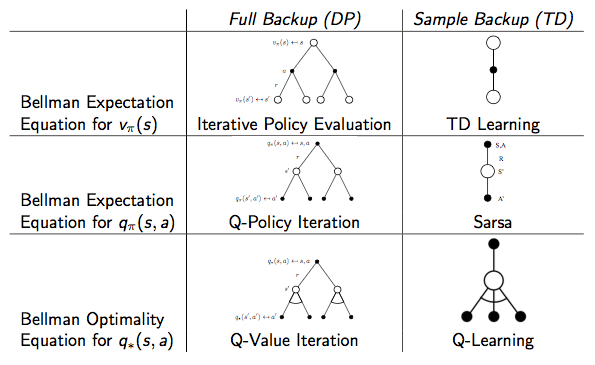
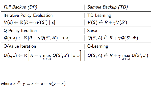
DP vs. TD

兩者的差別見下表：



Reference

[1] Reinforcement Learning: An Introduction, Richard S. Sutton and Andrew G. Barto, 2018

[2] David Silver's Homepage

作者：Poll的筆記

部落格出處：http://www.cnblogs.com/maybe2030/

本文版權歸作者和部落格園所有，歡迎轉載，轉載請标明出處。

<如果你覺得本文還不錯，對你的學習帶來了些許幫助，請幫忙點選右下角的推薦>