用圖機器學習探索 A 股個股相關性變化

在本系列的前文 [1,2]中，我們介紹了如何使用 Python 語言圖分析庫 NetworkX [3] + Nebula Graph

[4] 來進行<權力的遊戲>中人物關系圖譜分析。

在本文中我們将介紹如何使用 Java 語言的圖分析庫 JGraphT [5] 并借助繪圖庫 mxgraph [6] ，可視化探索 A 股的行業個股的相關性随時間的變化情況。

資料集的處理

本文主要分析方法參考了[7,8]，有兩種資料集：

股票資料（點集）

從 A 股中按股票代碼順序選取了 160 隻股票（排除摘牌或者 ST 的）。每一支股票都被模組化成一個點，每個點的屬性有股票代碼，股票名稱，以及證監會對該股票對應上市公司所屬闆塊分類等三種屬性；

表1：點集示例

頂點id	股票代碼	股票名稱	所屬闆塊
1	SZ0001	平安銀行	金融行業
2	600000	浦發銀行
3	600004	白雲機場	交通運輸
4	600006	東風汽車	汽車制造
5	600007	中國國貿	開發區
6	600008	首創股份	環保行業
7	600009	上海機場
8	600010	包鋼股份	鋼鐵行業

股票關系（邊集）

邊隻有一個屬性，即權重。邊的權重代表邊的源點和目标點所代表的兩支股票所屬上市公司業務上的的相似度——相似度的具體計算方法參考 [7,8]：取一段時間（2014 年 1 月 1 日 - 2020 年 1 月 1 日）内，個股的日收益率的時間序列相關性 $P_{ij}$ 再定義個股之間的距離為 (也即兩點之間的邊權重）：

$$l_{ij} = sqrt{2（1-P_{ij}）}$$

通過這樣的處理，距離取值範圍為 [0,2]。這意味着距離越遠的個股，兩個之間的收益率相關性越低。

表2：邊集示例

邊的源點 ID	邊的目标點 ID	邊的權重
11	12	0.493257968
22	83	0.517027513
23	78	0.606206233
		0.653692415
		0.677631482
	27	0.695705171
		0.71124344
		0.73581915
	18	0.771556458
		0.785046446
9	20	0.789606527
		0.796009627
25	63	0.797218349
	72	0.799230001
	115	0.803534952

這樣的點集和邊集構成一個圖網絡，可以将這個網絡存儲在圖資料庫

中。

JGraphT

JGraphT 是一個開放源代碼的 Java 類庫，它不僅為我們提供了各種高效且通用的圖資料結構，還為解決最常見的圖問題提供了許多有用的算法：

支援有向邊、無向邊、權重邊、非權重邊等；
支援簡單圖、多重圖、僞圖；
提供了用于圖周遊的專用疊代器（DFS，BFS）等；
提供了大量常用的的圖算法，如路徑查找、同構檢測、着色、公共祖先、遊走、連通性、比對、循環檢測、分區、切割、流、中心性等算法；
可以友善地導入 / 導出 GraphViz [9]。導出的 GraphViz 可被導入可視化工具 Gephi[10] 進行分析與展示；
可以友善地使用其他繪圖元件，如：JGraphX，mxGraph，Guava Graphs Generators 等工具繪制出圖網絡。

下面，我們來實踐一把，先在 JGraphT 中建立一個有向圖：

import org.jgrapht.*;
import org.jgrapht.graph.*;
import org.jgrapht.nio.*;
import org.jgrapht.nio.dot.*;
import org.jgrapht.traverse.*;

import java.io.*;
import java.net.*;
import java.util.*;

Graph<URI, DefaultEdge> g = new DefaultDirectedGraph<>(DefaultEdge.class);

添加頂點：

URI google = new URI("http://www.google.com");
URI wikipedia = new URI("http://www.wikipedia.org");
URI jgrapht = new URI("http://www.jgrapht.org");

// add the vertices
g.addVertex(google);
g.addVertex(wikipedia);
g.addVertex(jgrapht);

添加邊：

// add edges to create linking structure
g.addEdge(jgrapht, wikipedia);
g.addEdge(google, jgrapht);
g.addEdge(google, wikipedia);
g.addEdge(wikipedia, google);

圖資料庫 Nebula Graph Database

JGraphT 通常使用本地檔案作為資料源，這在靜态網絡研究的時候沒什麼問題，但如果圖網絡經常會發生變化——例如，股票資料每日都在變化——每次生成全新的靜态檔案再加載分析就有些麻煩，最好整個變化過程可以持久化地寫入一個資料庫中，并且可以實時地直接從資料庫中加載子圖或者全圖做分析。本文選用

作為存儲圖資料的圖資料庫。

Nebula Graph 的 Java 用戶端 Nebula-Java [11] 提供了兩種通路 Nebula Graph 方式：一種是通過圖查詢語言 nGQL [12] 與查詢引擎層 [13] 互動，這通常适用于有複雜語義的子圖通路類型; 另一種是通過 API 與底層的存儲層（storaged）[14] 直接互動，用于擷取全量的點和邊。除了可以通路

本身外，Nebula-Java 還提供了與 Neo4j [15]、JanusGraph [16]、Spark [17] 等互動的示例。

在本文中，我們選擇直接通路存儲層（storaged）來擷取全部的點和邊。下面兩個接口可以用來讀取所有的點、邊資料：

// space 為待掃描的圖空間名稱，returnCols 為需要讀取的點/邊及其屬性列，
// returnCols 參數格式：{tag1Name: prop1, prop2, tag2Name: prop3, prop4, prop5}
Iterator<ScanVertexResponse> scanVertex(
            String space, Map<String, List<String>> returnCols);
Iterator<ScanEdgeResponse> scanEdge(
            String space, Map<String, List<String>> returnCols);

第一步：初始化一個用戶端，和一個 ScanVertexProcessor。ScanVertexProcessor 用來對讀出來的頂點資料進行解碼：

MetaClientImpl metaClientImpl = new MetaClientImpl(metaHost, metaPort);
metaClientImpl.connect();
StorageClient storageClient = new StorageClientImpl(metaClientImpl);
Processor processor = new ScanVertexProcessor(metaClientImpl);

第二步：調用 scanVertex 接口，該接口會傳回一個 scanVertexResponse 對象的疊代器：

Iterator<ScanVertexResponse> iterator =
                storageClient.scanVertex(spaceName, returnCols);

第三步：不斷讀取該疊代器所指向的 scanVertexResponse 對象中的資料，直到讀取完所有資料。讀取出來的頂點資料先儲存起來，後面會将其添加到到 JGraphT 的圖結構中：

while (iterator.hasNext()) {
  ScanVertexResponse response = iterator.next();
  if (response == null) {
    log.error("Error occurs while scan vertex");
    break;
  }
  
  Result result =  processor.process(spaceName, response);
  results.addAll(result.getRows(TAGNAME));
}

讀取邊資料的方法和上面的流程類似。

在 JGraphT 中進行圖分析

第一步：在 JGraphT 中建立一個無向權重圖 graph：

Graph<String, MyEdge> graph = GraphTypeBuilder
                .undirected()
    .weighted(true)
    .allowingMultipleEdges(true)
    .allowingSelfLoops(false)
    .vertexSupplier(SupplierUtil.createStringSupplier())
    .edgeSupplier(SupplierUtil.createSupplier(MyEdge.class))
    .buildGraph();

第二步：将上一步從 Nebula Graph 圖空間中讀出來的點、邊資料添加到 graph 中：

for (VertexDomain vertex : vertexDomainList){
    graph.addVertex(vertex.getVid().toString());
    stockIdToName.put(vertex.getVid().toString(), vertex);
}

for (EdgeDomain edgeDomain : edgeDomainList){
    graph.addEdge(edgeDomain.getSrcid().toString(), edgeDomain.getDstid().toString());
    MyEdge newEdge = graph.getEdge(edgeDomain.getSrcid().toString(), edgeDomain.getDstid().toString());
    graph.setEdgeWeight(newEdge, edgeDomain.getWeight());
}

第三步：參考 [7,8] 中的分析法，對剛才的圖 graph 使用 Prim 最小生成樹算法（minimun-spanning-tree），并調用封裝好的 drawGraph 接口畫圖：

普裡姆算法（Prim's algorithm），圖論中的一種算法，可在權重連通圖裡搜尋最小生成樹。即，由此算法搜尋到的邊子集所構成的樹中，不但包括了連通圖裡的所有頂點，且其所有邊的權值之和亦為最小。

SpanningTreeAlgorithm.SpanningTree pMST = new PrimMinimumSpanningTree(graph).getSpanningTree();

Legend.drawGraph(pMST.getEdges(), filename, stockIdToName);

第四步：drawGraph 方法封裝了畫圖的布局等各項參數設定。這個方法将同一闆塊的股票渲染為同一顔色，将距離接近的股票排列聚集在一起。

public class Legend {
  
...
  
  public static void drawGraph(Set<MyEdge> edges, String filename, Map<String, VertexDomain> idVertexMap) throws IOException {
     // Creates graph with model
     mxGraph graph = new mxGraph();
     Object parent = graph.getDefaultParent();

     // set style
     graph.getModel().beginUpdate();
     mxStylesheet myStylesheet =  graph.getStylesheet();
     graph.setStylesheet(setMsStylesheet(myStylesheet));

     Map<String, Object> idMap = new HashMap<>();
     Map<String, String> industryColor = new HashMap<>();

     int colorIndex = 0;

     for (MyEdge edge : edges) {
       Object src, dst;
       if (!idMap.containsKey(edge.getSrc())) {
         VertexDomain srcNode = idVertexMap.get(edge.getSrc());
         String nodeColor;
         if (industryColor.containsKey(srcNode.getIndustry())){
           nodeColor = industryColor.get(srcNode.getIndustry());
         }else {
           nodeColor = COLOR_LIST[colorIndex++];
           industryColor.put(srcNode.getIndustry(), nodeColor);
         }
         src = graph.insertVertex(parent, null, srcNode.getName(), 0, 0, 105, 50, "fillColor=" + nodeColor);
         idMap.put(edge.getSrc(), src);
       } else {
         src = idMap.get(edge.getSrc());
       }

       if (!idMap.containsKey(edge.getDst())) {
         VertexDomain dstNode = idVertexMap.get(edge.getDst());

         String nodeColor;
         if (industryColor.containsKey(dstNode.getIndustry())){
           nodeColor = industryColor.get(dstNode.getIndustry());
         }else {
           nodeColor = COLOR_LIST[colorIndex++];
           industryColor.put(dstNode.getIndustry(), nodeColor);
         }

         dst = graph.insertVertex(parent, null, dstNode.getName(), 0, 0, 105, 50, "fillColor=" + nodeColor);
         idMap.put(edge.getDst(), dst);
       } else {
         dst = idMap.get(edge.getDst());
       }
       graph.insertEdge(parent, null, "", src, dst);
     }


     log.info("vertice " + idMap.size());
     log.info("colorsize " + industryColor.size());

     mxFastOrganicLayout layout = new mxFastOrganicLayout(graph);
     layout.setMaxIterations(2000);
     //layout.setMinDistanceLimit(10D);
     layout.execute(parent);

     graph.getModel().endUpdate();

     // Creates an image than can be saved using ImageIO
     BufferedImage image = createBufferedImage(graph, null, 1, Color.WHITE,
                                               true, null);

     // For the sake of this example we display the image in a window
     // Save as JPEG
     File file = new File(filename);
     ImageIO.write(image, "JPEG", file);

   }
  
  ...
    
}

第五步：生成可視化：

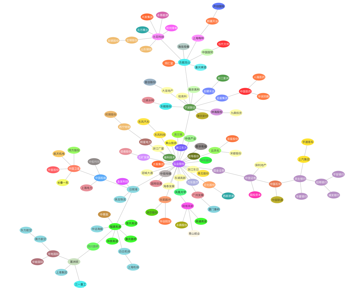
圖1中每個頂點的顔色代表證監會對該股票所屬上市公司歸類的闆塊。

可以看到，實際業務近似度較高的股票已經聚攏成簇狀（例如：高速闆塊、銀行版本、機場航空闆塊），但也會有部分關聯性不明顯的個股被聚類在一起，具體原因需要單獨進行個股研究。

圖1：基于 2015-01-01 至 2020-01-01 的股票資料計算出的聚集性

第六步：基于不同時間視窗的一些其他動态探索

上節中，結論主要基于 2015-01-01 到 2020-01-01 的個股聚集性。這一節我們還做了一些其他的嘗試：以 2 年為一個時間滑動視窗，分析方法不變，定性探索聚叢集是否随着時間變化會發生改變。

圖2：基于 2014-01-01 至 2016-01-01 的股票資料計算出的聚集性

圖3：基于 2015-01-01 至 2017-01-01 的股票資料計算出的聚集性

圖4：基于 2016-01-01 至 2018-01-01 的股票資料計算出的聚集性

圖5：基于 2017-01-01 至 2019-01-01 的股票資料計算出的聚集性

圖6：基于 2018-01-01 至 2020-01-01 的股票資料計算出的聚集性

粗略分析看，随着時間視窗變化，有些闆塊（高速、銀行、機場航空、房産、能源）的闆塊内部個股聚集性一直保持比較好——這意味着随着時間變化，這個版塊内各種一直保持比較高的相關性；但有些闆塊（制造）的聚集性會持續變化——意味着相關性一直在發生變化。

Disclaim

本文不構成任何投資建議，且作者不持有本文中任一股票。

受限于停牌、熔斷、漲跌停、送轉、并購、主營業務變更等情況，資料處理可能有錯誤，未做一一檢查。

受時間所限，本文隻選用了 160 個個股樣本過去 6 年的資料，隻采用了最小擴張樹一種辦法來做聚類分類。未來可以使用更大的資料集（例如美股、衍生品、數字貨币），嘗試更多種圖機器學習的辦法。

本文代碼可見[18]

Reference

[1] 用 NetworkX + Gephi + Nebula Graph 分析<權力的遊戲>人物關系（上篇）

https://nebula-graph.com.cn/posts/game-of-thrones-relationship-networkx-gephi-nebula-graph/

[2] 用 NetworkX + Gephi + Nebula Graph 分析<權力的遊戲>人物關系（下篇）

https://nebula-graph.com.cn/posts/game-of-thrones-relationship-networkx-gephi-nebula-graph-part-two/

[3] NetworkX: a Python package for the creation, manipulation, and study of the structure, dynamics, and functions of complex networks.

https://networkx.github.io/

[4] Nebula Graph: A powerfully distributed, scalable, lightning-fast graph database written in C++.

https://nebula-graph.io/

[5] JGraphT: a Java library of graph theory data structures and algorithms.

https://jgrapht.org/

[6] mxGraph: JavaScript diagramming library that enables interactive graph and charting applications.

https://jgraph.github.io/mxgraph/

[7] Bonanno, Giovanni & Lillo, Fabrizio & Mantegna, Rosario. (2000). High-frequency Cross-correlation in a Set of Stocks. arXiv.org, Quantitative Finance Papers. 1. 10.1080/713665554.

[8] Mantegna, R.N. Hierarchical structure in financial markets. Eur. Phys. J. B 11, 193–197 (1999).

[9]

https://graphviz.org/

[10]

https://gephi.org/

[11]

https://github.com/vesoft-inc/nebula-java

[12] Nebula Graph Query Language (nGQL).

https://docs.nebula-graph.io/manual-EN/1.overview/1.concepts/2.nGQL-overview/

[13] Nebula Graph Query Engine.

https://github.com/vesoft-inc/nebula-graph

[14] Nebula-storage: A distributed consistent graph storage.