在 VGG 網絡論文研讀中,我們了解到卷積神經網絡也可以進行到很深層,VGG16 和 VGG19 就是證明。但卷積網絡變得更深呢?當然是可以的。深度神經網絡能夠從提取圖像各個層級的特征,使得圖像識别的準确率越來越高。但在2014年和15年那會兒,将卷積網絡變深且取得不錯的訓練效果并不是一件容易的事。
深度卷積網絡一開始面臨的最主要的問題是梯度消失和梯度爆炸。那什麼是梯度消失和梯度爆炸呢?所謂梯度消失,就是在深層神經網絡的訓練過程中,計算得到的梯度越來越小,使得權值得不到更新的情形,這樣算法也就失效了。而梯度爆炸則是相反的情況,是指在神經網絡訓練過程中梯度變得越來越大,權值得到瘋狂更新的情形,這樣算法得不到收斂,模型也就失效了。當然,其間通過設定
relu
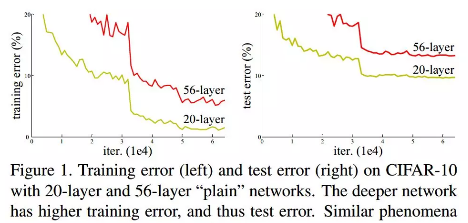
由上圖我們可以看到 56 層的普通卷積網絡不管是在訓練集還是測試集上的訓練誤差都要高于 20 層的卷積網絡。是個典型的退化現象。
這退化問題不解決,咱們的深度學習就無法 go deeper. 于是何凱明等一幹大佬就發明了今天我們要研讀的論文主題——殘差網絡 ResNet.
殘差塊與殘差網絡
要了解殘差網絡,就必須了解殘差塊(residual block)這個結構,因為殘差塊是殘差網絡的基本組成部分。回憶一下我們之前學到的各種卷積網絡結構(LeNet-5/AlexNet/VGG),通常結構就是卷積池化再卷積池化,中間的卷積池化操作可以很多層。類似這樣的網絡結構何凱明在論文中将其稱為普通網絡(Plain Network),何凱明認為普通網絡解決不了退化問題,我們需要在網絡結構上作出創新。
何凱明給出的創新在于給網絡之間添加一個捷徑(shortcuts)或者也叫跳躍連接配接(skip connection),這使得捷徑之間之間的網絡能夠學習一個恒等函數,使得在加深網絡的情形下訓練效果至少不會變差。殘差塊的基本結構如下:

X
F(X)
X
relu
F(X)
F(X)+X
。當很多個具備類似結構的這樣的殘差塊組建到一起時,殘差網絡就順利形成了。殘差網絡能夠順利訓練很深層的卷積網絡,其中能夠很好的解決網絡的退化問題。
或許你可能會問憑什麼加了一條從輸入到輸出的捷徑網絡就能防止退化訓練更深層的卷積網絡?或是是說殘差網絡為什麼能有效?我們将上述殘差塊的兩層輸入輸出符号改為 和 ,相應的就有:
W
是很容易衰減為零的,假設偏置同樣為零的情形下就有 = 。深度學習的試驗表明學習這個恒等式并不困難,這就意味着,在擁有跳躍連接配接的普通網絡即使多加幾層,其效果也并不遜色于加深之前的網絡效果。當然,我們的目标不是保持網絡不退化,而是需要提升網絡表現,當隐藏層能夠學到一些有用的資訊時,殘差網絡的效果就會提升。是以,殘差網絡之是以有效是在于它能夠很好的學習上述那個恒等式,而普通網絡學習恒等式都很困難,殘差網絡在兩者相較中自然勝出。
由很多個殘差塊組成的殘差網絡如下圖右圖所示:
Identity Block
Convolutional Block
,顧名思義,就是跳躍連接配接中包含卷積操作,用來使得輸入輸出一緻。且看二者的 keras 實作方法。
Identity Block 的圖示如下:
def identity_block(X, f, filters, stage, block):
"""
Implementation of the identity block as defined in Figure 3
Arguments:
X -- input tensor of shape (m, n_H_prev, n_W_prev, n_C_prev)
f -- integer, specifying the shape of the middle CONV's window for the main path
filters -- python list of integers, defining the number of filters in the CONV layers of the main path
stage -- integer, used to name the layers, depending on their position in the network
Returns:
block -- string/character, used to name the layers, depending on their position in the network

 X -- output of the identity block, tensor of shape (n_H, n_W, n_C)
""" # defining name basis
conv_name_base = 'res' + str(stage) + block + '_branch'
bn_name_base = 'bn' + str(stage) + block + '_branch' # Retrieve Filters
F1, F2, F3 = filters
# Save the input value. You'll need this later to add back to the main path.
X_shortcut = X
# First component of main path
X = Conv2D(filters = F1, kernel_size = (1, 1), strides = (1,1), padding = 'valid', name = conv_name_base + '2a', kernel_initializer = glorot_uniform(seed=0))(X)
X = BatchNormalization(axis = 3, name = bn_name_base + '2a')(X)
X = Activation('relu')(X)
# Second component of main path
X = Conv2D(filters = F2, kernel_size = (f, f), strides= (1, 1), padding = 'same', name = conv_name_base + '2b', kernel_initializer = glorot_uniform(seed=0))(X)
X = BatchNormalization(axis = 3, name = bn_name_base + '2b')(X)
X = Activation('relu')(X)
# Third component of main path
X = Conv2D(filters = F3, kernel_size = (1, 1), strides = (1, 1), padding = 'valid', name = conv_name_base + '2c', kernel_initializer = glorot_uniform(seed=0))(X)
X = BatchNormalization(axis = 3, name = bn_name_base + '2c')(X)
# Final step: Add shortcut value to main path, and pass it through a RELU activation
X = Add()([X, X_shortcut])
X = Activation('relu')(X)
return X
可見殘差塊的實作特殊之處就在于添加一條跳躍連接配接。
Convolutional Block 的圖示如下:
def convolutional_block(X, f, filters, stage, block, s = 2):
"""
Implementation of the convolutional block as defined in Figure 4
Arguments:
f -- integer, specifying the shape of the middle CONV's window for the main path
X -- input tensor of shape (m, n_H_prev, n_W_prev, n_C_prev)
filters -- python list of integers, defining the number of filters in the CONV layers of the main path
stage -- integer, used to name the layers, depending on their position in the network
X -- output of the convolutional block, tensor of shape (n_H, n_W, n_C)
block -- string/character, used to name the layers, depending on their position in the network
 s -- Integer, specifying the stride to be used

 Returns:
""" # defining name basis
conv_name_base = 'res' + str(stage) + block + '_branch'
bn_name_base = 'bn' + str(stage) + block + '_branch' # Retrieve Filters
F1, F2, F3 = filters
# Save the input value
X_shortcut = X
##### MAIN PATH ##### # First component of main path
X = Conv2D(filters = F1, kernel_size = (1, 1), strides = (s,s), padding = 'valid', name = conv_name_base + '2a', kernel_initializer = glorot_uniform(seed=0))(X)
X = BatchNormalization(axis = 3, name = bn_name_base + '2a')(X)
X = Activation('relu')(X)
# Second component of main path
X = Conv2D(filters = F2, kernel_size = (f, f), strides = (1,1), padding = 'same', name = conv_name_base + '2b', kernel_initializer = glorot_uniform(seed=0))(X)
X = BatchNormalization(axis = 3, name = bn_name_base + '2b')(X)
X = Activation('relu')(X)
# Third component of main path
X = Conv2D(filters = F3, kernel_size = (1, 1), strides = (1,1), padding = 'valid', name = conv_name_base + '2c', kernel_initializer = glorot_uniform(seed=0))(X)
X = BatchNormalization(axis = 3, name = bn_name_base + '2c')(X)
##### SHORTCUT PATH ####
X_shortcut = Conv2D(filters = F3, kernel_size = (1, 1), strides = (s, s), padding = 'valid', name = conv_name_base + '1', kernel_initializer = glorot_uniform(seed=0))(X_shortcut)
X_shortcut = BatchNormalization(axis = 3, name = bn_name_base + '1')(X_shortcut)
# Final step: Add shortcut value to main path, and pass it through a RELU activation
X = Add()([X, X_shortcut])
X = Activation('relu')(X)
return X
殘差網絡 resnet50 的 keras 實作
搭建好元件殘差塊之後就是确定網絡結構,将一個個殘差塊組成殘差網絡。下面搭建一個 resnet50 的殘差網絡,其基本結構如下:
CONV2D -> BATCHNORM -> RELU -> MAXPOOL -> CONVBLOCK -> IDBLOCK2 -> CONVBLOCK -> IDBLOCK3 -> CONVBLOCK -> IDBLOCK5 -> CONVBLOCK -> IDBLOCK2 -> AVGPOOL -> TOPLAYER
def ResNet50(input_shape = (64, 64, 3), classes = 6):
# Define the input as a tensor with shape input_shape
X_input = Input(input_shape)
# Zero-Padding
X = ZeroPadding2D((3, 3))(X_input)
# Stage 1
X = Conv2D(64, (7, 7), strides = (2, 2), name = 'conv1', kernel_initializer = glorot_uniform(seed=0))(X)
X = BatchNormalization(axis = 3, name = 'bn_conv1')(X)
X = Activation('relu')(X)
X = MaxPooling2D((3, 3), strides=(2, 2))(X)
# Stage 2
X = convolutional_block(X, f = 3, filters = [64, 64, 256], stage = 2, block='a', s = 1)
X = identity_block(X, 3, [64, 64, 256], stage=2, block='b')
X = identity_block(X, 3, [64, 64, 256], stage=2, block='c')
# Stage 3
X = convolutional_block(X, f = 3, filters = [128, 128, 512], stage = 3, block='a', s = 2)
X = identity_block(X, 3, [128, 128, 512], stage=3, block='b')
X = identity_block(X, 3, [128, 128, 512], stage=3, block='c')
X = identity_block(X, 3, [128, 128, 512], stage=3, block='d')
# Stage 4
X = convolutional_block(X, f = 3, filters = [256, 256, 1024], stage = 4, block='a', s = 2)
X = identity_block(X, 3, [256, 256, 1024], stage=4, block='b')
X = identity_block(X, 3, [256, 256, 1024], stage=4, block='c')
X = identity_block(X, 3, [256, 256, 1024], stage=4, block='d')
X = identity_block(X, 3, [256, 256, 1024], stage=4, block='e')
X = identity_block(X, 3, [256, 256, 1024], stage=4, block='f')
# Stage 5
X = convolutional_block(X, f = 3, filters = [512, 512, 2048], stage = 5, block='a', s = 2)
X = identity_block(X, 3, [512, 512, 2048], stage=5, block='b')
X = identity_block(X, 3, [512, 512, 2048], stage=5, block='c')
# AVGPOOL (≈1 line). Use "X = AveragePooling2D(...)(X)"
X = AveragePooling2D((2, 2), strides=(2, 2))(X)
# output layer
X = Flatten()(X)
X = Dense(classes, activation='softmax', name='fc' + str(classes), kernel_initializer = glorot_uniform(seed=0))(X)
# Create model
model = Model(inputs = X_input, outputs = X, name='ResNet50')
return model
這樣一個 resnet50 的殘差網絡就搭建好了,其關鍵還是在于搭建殘差塊,殘差塊搭建好之後隻需根據網絡結構建構殘差網絡即可。當然,其間也可以看到 keras 作為一個優秀的深度學習架構的便利之處。
原文釋出時間為:2018-10-13
本文作者:louwill
本文來自雲栖社群合作夥伴“
Python愛好者社群”,了解相關資訊可以關注“
”。