了解mulitband。所謂的mulitband,其實就是一種多尺度的樣條融合,其實作的主要方法就是laplace金字塔。高斯金字塔是向下采樣,而laplace金字塔式向上采樣(也就是恢複),采用的都是內插補點的方法。如何能夠在金字塔各個層次上面進行圖像的融合,結果證明是相當不錯的。網絡上面流傳的一個類解釋了這個問題,并且能夠拿來用:
#
include
"stdafx.h"
#
include
<iostream>
#
include
<vector>
#
include
<opencv2/core/core.hpp>
#
include
<opencv2/imgproc/imgproc.hpp>
#
include
<opencv2/highgui/highgui.hpp>
#
include
<opencv2/features2d/features2d.hpp>
#
include
<opencv2/calib3d/calib3d.hpp>
using
namespace
cv;
#
ifdef
_DEBUG
#
define
new
DEBUG_NEW
#
endif
#
define
DllExport _declspec (dllexport)
/*
1.設計一個mask(一半全1,一半全0),并計算level層的gaussion_mask[i];
2.計算兩幅圖像每一層的Laplacian[i],并與gaussion_mask[i]相乘,合成一幅result_lapacian[i];
3.對兩幅圖像不斷求prydown,并把最高層儲存在gaussion[i],與gaussion_mask[i]相乘,合成一幅result_gaussion;
4,對result_gaussion不斷求pryup,每一層都與result_lapacian[i]合成,最後得到原-圖像大小的融合圖像。
*/
class
LaplacianBlending {
private
:
Mat_<Vec3f> top;
Mat_<Vec3f> down;
Mat_<
float
> blendMask;
vector<Mat_<Vec3f> > topLapPyr,downLapPyr,resultLapPyr; //Laplacian Pyramids
Mat topHighestLevel, downHighestLevel, resultHighestLevel;
vector<Mat_<Vec3f> > maskGaussianPyramid; //masks are 3-channels for easier multiplication with RGB
int
levels;
//建立金字塔
void
buildPyramids() {
buildLaplacianPyramid(top,topLapPyr,topHighestLevel);
buildLaplacianPyramid(down,downLapPyr,downHighestLevel);
buildGaussianPyramid();
}
//建立gauss金字塔
void
buildGaussianPyramid() {//金字塔内容Y為a每一層的掩模
assert(topLapPyr.size()>0);
maskGaussianPyramid.clear();
Mat currentImg;
//blendMask就是掩碼
cvtColor(blendMask, currentImg, CV_GRAY2BGR); //store color img of blend mask into maskGaussianPyramid
maskGaussianPyramid.push_back(currentImg); //0-level
currentImg = blendMask;
for
(
int
l=1; l<levels+1; l++) {
Mat _down;
if
(topLapPyr.size() > l)
pyrDown(currentImg, _down, topLapPyr[l].size());
else
pyrDown(currentImg, _down, topHighestLevel.size()); //lowest level
Mat down;
cvtColor(_down, down, CV_GRAY2BGR);
maskGaussianPyramid.push_back(down); //add color blend mask into mask Pyramid
currentImg = _down;
}
}
//建立laplacian金字塔
void
buildLaplacianPyramid(
const
Mat& img, vector<Mat_<Vec3f> >& lapPyr, Mat& HighestLevel) {
lapPyr.clear();
Mat currentImg = img;
for
(
int
l=0; l<levels; l++) {
Mat down,up;
pyrDown(currentImg, down);
pyrUp(down, up,currentImg.size());
Mat lap = currentImg - up; //存儲的就是殘D差
lapPyr.push_back(lap);
currentImg = down;
}
currentImg.copyTo(HighestLevel);
}
Mat_<Vec3f> reconstructImgFromLapPyramid() {
//将左右laplacian圖像拼成的resultLapPyr金字塔中每一層
//從上到下插值放大并相加,即得blend圖像結果
Mat currentImg = resultHighestLevel;
for
(
int
l=levels-1; l>=0; l--) {
Mat up;
pyrUp(currentImg, up, resultLapPyr[l].size());
currentImg = up + resultLapPyr[l];
}
return
currentImg;
}
void
blendLapPyrs() {
//獲得每層金字塔中直接用左右兩圖Laplacian變換拼成的圖像
//一半的一半就是在這個地方計算的。 是基于掩模的方式進行的.
resultHighestLevel = topHighestLevel.mul(maskGaussianPyramid.back()) +
downHighestLevel.mul(Scalar(1.0,1.0,1.0) - maskGaussianPyramid.back());
for
(
int
l=0; l<levels; l++) {
Mat A = topLapPyr[l].mul(maskGaussianPyramid[l]);
Mat antiMask = Scalar(1.0,1.0,1.0) - maskGaussianPyramid[l];
Mat B = downLapPyr[l].mul(antiMask);
Mat_<Vec3f> blendedLevel = A + B;
resultLapPyr.push_back(blendedLevel);
}
}
public
:
LaplacianBlending(
const
Mat_<Vec3f>& _top,
const
Mat_<Vec3f>& _down,
const
Mat_<
float
>& _blendMask,
int
_levels)://預設數y據Y,使1用 LaplacianBlending lb(l,r,m,4);
top(_top),down(_down),blendMask(_blendMask),levels(_levels)
{
assert(_top.size() == _down.size());
assert(_top.size() == _blendMask.size());
buildPyramids(); //建立laplacian金字塔和gauss金字塔
blendLapPyrs(); //将左右金字塔融合成為a一個圖檔
};
Mat_<Vec3f> blend() {
return
reconstructImgFromLapPyramid();//reconstruct Image from Laplacian Pyramid
}
};
Mat_<Vec3f> LaplacianBlend(
const
Mat_<Vec3f>& t,
const
Mat_<Vec3f>& d,
const
Mat_<
float
>& m) {
LaplacianBlending lb(t,d,m,4);
return
lb.blend();
}
DllExport
double
aValue =1.5;
DllExport
int
dlladd()
{
return
5;
}
DllExport
int
dlladd(
int
a,
int
b)
{
return
a+b;
}
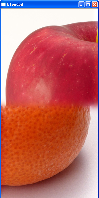
DllExport cv::Mat imagetest()
{
cv::Mat image1= cv::imread( "C:\\apple.png",1);
cv::Mat image2= cv::imread( "C:\\orange.png",1);
Mat_<Vec3f> t; image1.convertTo(t,CV_32F,1.0/255.0); //Vec3f表示有三個通道,即 [row][column][depth]
Mat_<Vec3f> d; image2.convertTo(d,CV_32F,1.0/255.0);
Mat_<
float
> m(t.rows,d.cols,0.0); //将m全部賦3值為a0
//m(Range::all(),Range(0,m.cols/2)) = 1.0; //原來初始的掩碼是在這裡
m(Range(0,m.rows/2),Range::all())=1.0;
Mat_<Vec3f> blend = LaplacianBlend(t,d, m);
imshow( "blended",blend);
return
blend;
}
需要注意的是, m(Range(0,m.rows/2),Range::all())=1.0表明了原始圖像的掩碼,這個掩碼就是那個分界的地方。
比如比如:
;

永達實際的項目上面,應該是這樣。
在使用這種方法進行大規模拼接的時候,主要是兩個問題
一個是效果,在上面的那個橘子蘋果的例子中,隻有前景的顔色有變化,實際上其它幾個地方色彩亮度變化不是很大。但是對于實際情況下的拼接來說,亮度有變化,比較難以處理。
二是效率。laplacian需要大量的過程,造成結果記憶體的需求很大,一時半會很難優化好。multband看來隻能夠在符合要求的簡單拼接中去實作使用。
來自為知筆記(Wiz)目前方向:圖像拼接融合、圖像識别
聯系方式:[email protected]