文本分類應該是自然語言進行中最普遍的一個應用,例如文章自動分類、郵件自動分類、垃圾郵件識别、使用者情感分類等等,在生活中有很多例子,這篇文章主要從傳統和深度學習兩塊來解釋下我們如何做一個文本分類器。
傳統的文本方法的主要流程是人工設計一些特征,從原始文檔中提取特征,然後指定分類器如LR、SVM,訓練模型對文章進行分類,比較經典的特征提取方法如頻次法、tf-idf、互資訊方法、N-Gram。
深度學習火了之後,也有很多人開始使用一些經典的模型如CNN、LSTM這類方法來做特征的提取, 這篇文章會比較粗地描述下,在文本分類的一些實驗
這裡主要描述兩種特征提取方法:頻次法、tf-idf、互資訊、N-Gram。
頻次法,顧名思義,十分簡單,記錄每篇文章的次數分布,然後将分布輸入機器學習模型,訓練一個合适的分類模型,對這類資料進行分類,需要指出的時,在統計次數分布時,可合理提出假設,頻次比較小的詞對文章分類的影響比較小,是以我們可合理地假設門檻值,濾除頻次小于門檻值的詞,減少特征空間次元。
TF-IDF相對于頻次法,有更進一步的考量,詞出現的次數能從一定程度反應文章的特點,即TF,而TF-IDF,增加了所謂的反文檔頻率,如果一個詞在某個類别上出現的次數多,而在全部文本上出現的次數相對比較少,我們認為這個詞有更強大的文檔區分能力,TF-IDF就是綜合考慮了頻次和反文檔頻率兩個因素。
互資訊方法也是一種基于統計的方法,計算文檔中出現詞和文檔類别的相關程度,即互資訊
基于N-Gram的方法是把文章序列,通過大小為N的視窗,形成一個個Group,然後對這些Group做統計,濾除出現頻次較低的Group,把這些Group組成特征空間,傳入分類器,進行分類。
最普通的基于CNN的方法就是Keras上的example做情感分析,接Conv1D,指定大小的window size來周遊文章,加上一個maxpool,如此多接入幾個,得到特征表示,然後加上FC,進行最終的分類輸出。
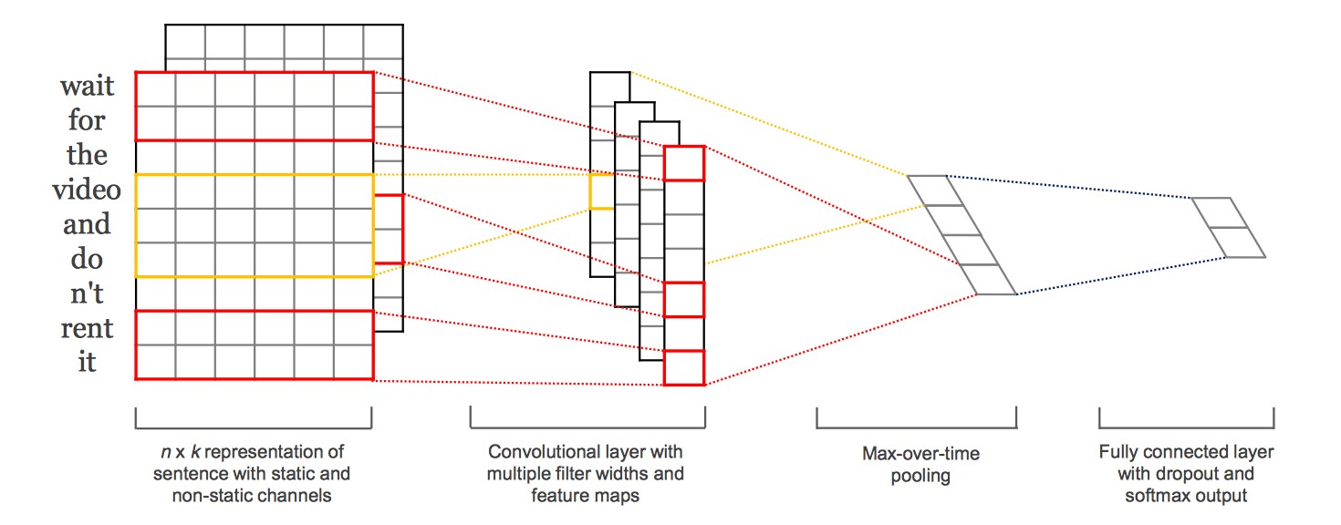
基于CNN的文本分類方法,最出名的應該是2014 Emnlp的 Convolutional Neural Networks for Sentence Classification,使用不同filter的cnn網絡,然後加入maxpool, 然後concat到一起。
這類CNN的方法,通過設計不同的window size來模組化不同尺度的關系,但是很明顯,丢失了大部分的上下文關系,Recurrent Convolutional Neural Networks for Text Classification,将每一個詞形成向量化表示時,加上上文和下文的資訊,每一個詞的表示如下:

整個結構架構如下:
如針對這句話”A sunset stroll along the South Bank affords an array of stunning vantage points”,stroll的表示包括c_l(stroll),pre_word2vec(stroll),c_r(stroll), c_l(stroll)編碼A sunset的語義,而c_r(stroll)編碼along the South Bank affords an array of stunning vantage points的資訊,每一個詞都如此處理,是以會避免普通cnn方法的上下文缺失的資訊。基于LSTM的方法
和基于CNN的方法中第一種類似,直接暴力地在embedding之後加入LSTM,然後輸出到一個FC進行分類,基于LSTM的方法,我覺得這也是一種特征提取方式,可能比較偏向模組化時序的特征;
在暴力的方法之上,A C-LSTM Neural Network for Text Classification,将embedding輸出不直接接入LSTM,而是接入到cnn,通過cnn得到一些序列,然後吧這些序列再接入到LSTM,文章說這麼做會提高最後分類的準去率。代碼實踐語料及任務介紹訓練的語料來自于大概31個新聞類别的新聞語料,但是其中有一些新聞數目比較少,是以取了數量比較多的前20個新聞類比的新聞語料,每篇新聞稿字數從幾百到幾千不等,任務就是訓練合适的分類器然後将新聞分為不同類别:
BowBow對語料處理,得到tokens set:def __get_all_tokens(self):
""" get all tokens of the corpus
"""
fwrite = open(self.data_path.replace("all.csv","all_token.csv"), 'w')
with open(self.data_path, "r") as fread:
i = 0
# while True:
for line in fread.readlines():
try:
line_list = line.strip().split("\t")
label = line_list[0]
self.labels.append(label)
text = line_list[1]
text_tokens = self.cut_doc_obj.run(text)
self.corpus.append(' '.join(text_tokens))
self.dictionary.add_documents([text_tokens])
fwrite.write(label+"\t"+"\\".join(text_tokens)+"\n")
i+=1
except BaseException as e:
msg = traceback.format_exc()
print msg
print "=====>Read Done<======"
break
self.token_len = self.dictionary.__len__()
print "all token len "+ str(self.token_len)
self.num_data = i
fwrite.close()然後,tokens set 以頻率門檻值進行濾除,然後對每篇文章做處理來進行向量化:def __filter_tokens(self, threshold_num=10):
small_freq_ids = [tokenid for tokenid, docfreq in self.dictionary.dfs.items() if docfreq < threshold_num ]
self.dictionary.filter_tokens(small_freq_ids)
self.dictionary.compactify()
def vec(self):
""" vec: get a vec representation of bow
self.__get_all_tokens()
print "before filter, the tokens len: {0}".format(self.dictionary.__len__())
self.__filter_tokens()
print "After filter, the tokens len: {0}".format(self.dictionary.__len__())
self.bow = []
for file_token in self.corpus:
file_bow = self.dictionary.doc2bow(file_token)
self.bow.append(file_bow)
# write the bow vec into a file
bow_vec_file = open(self.data_path.replace("all.csv","bow_vec.pl"), 'wb')
pickle.dump(self.bow,bow_vec_file)
bow_vec_file.close()
bow_label_file = open(self.data_path.replace("all.csv","bow_label.pl"), 'wb')
pickle.dump(self.labels,bow_label_file)
bow_label_file.close()最終就得到每篇文章的bow的向量,由于這塊的代碼是在我的筆記本上運作的,直接跑占用記憶體太大,因為每一篇文章在token set中的表示是極其稀疏的,是以我們可以選擇将其轉為csr表示,然後進行模型訓練,轉為csr并儲存中間結果代碼如下:def to_csr(self):
self.bow = pickle.load(open(self.data_path.replace("all.csv","bow_vec.pl"), 'rb'))
self.labels = pickle.load(open(self.data_path.replace("all.csv","bow_label.pl"), 'rb'))
data = []
rows = []
cols = []
line_count = 0
for line in self.bow:
for elem in line:
rows.append(line_count)
cols.append(elem[0])
data.append(elem[1])
line_count += 1
print "dictionary shape ({0},{1})".format(line_count, self.dictionary.__len__())
bow_sparse_matrix = csr_matrix((data,(rows,cols)), shape=[line_count, self.dictionary.__len__()])
print "bow_sparse matrix shape: "
print bow_sparse_matrix.shape
# rarray=np.random.random(size=line_count)
self.train_set, self.test_set, self.train_tag, self.test_tag = train_test_split(bow_sparse_matrix, self.labels, test_size=0.2)
print "train set shape: "
print self.train_set.shape
train_set_file = open(self.data_path.replace("all.csv","bow_train_set.pl"), 'wb')
pickle.dump(self.train_set,train_set_file)
train_tag_file = open(self.data_path.replace("all.csv","bow_train_tag.pl"), 'wb')
pickle.dump(self.train_tag,train_tag_file)
test_set_file = open(self.data_path.replace("all.csv","bow_test_set.pl"), 'wb')
pickle.dump(self.test_set,test_set_file)
test_tag_file = open(self.data_path.replace("all.csv","bow_test_tag.pl"), 'wb')
pickle.dump(self.test_tag,test_tag_file)最後訓練模型代碼如下:def train(self):
print "Beigin to Train the model"
lr_model = LogisticRegression()
lr_model.fit(self.train_set, self.train_tag)
print "End Now, and evalution the model with test dataset"
# print "mean accuracy: {0}".format(lr_model.score(self.test_set, self.test_tag))
y_pred = lr_model.predict(self.test_set)
print classification_report(self.test_tag, y_pred)
print confusion_matrix(self.test_tag, y_pred)
print "save the trained model to lr_model.pl"
joblib.dump(lr_model, self.data_path.replace("all.csv","bow_lr_model.pl")) TF-IDFTF-IDF和Bow的操作十分類似,隻是在向量化使使用tf-idf的方法:def vec(self):
vectorizer = CountVectorizer(min_df=1e-5)
transformer = TfidfTransformer()
# sparse matrix
self.tfidf = transformer.fit_transform(vectorizer.fit_transform(self.corpus))
words = vectorizer.get_feature_names()
print "word len: {0}".format(len(words))
# print self.tfidf[0]
print "tfidf shape ({0},{1})".format(self.tfidf.shape[0], self.tfidf.shape[1])
# write the tfidf vec into a file
tfidf_vec_file = open(self.data_path.replace("all.csv","tfidf_vec.pl"), 'wb')
pickle.dump(self.tfidf,tfidf_vec_file)
tfidf_vec_file.close()
tfidf_label_file = open(self.data_path.replace("all.csv","tfidf_label.pl"), 'wb')
pickle.dump(self.labels,tfidf_label_file)
tfidf_label_file.close()這兩類方法效果都不錯,都能達到98+%的準确率。CNN語料處理的方法和傳統的差不多,分詞之後,使用pretrain 的word2vec,這裡我遇到一個坑,我開始對我的分詞太自信了,最後模型一直不能收斂,後來向我們組博士請教,極有可能是由于分詞的詞序列中很多在pretrained word2vec裡面是不存在的,而我這部分直接丢棄了,所有可能存在問題,分詞添加了詞典,然後,對于pre-trained word2vec不存在的詞做了一個随機初始化,然後就能收斂了,學習了!!!載入word2vec模型和建構cnn網絡代碼如下(增加了一些bn和dropout的手段):def gen_embedding_matrix(self, load4file=True):
""" gen_embedding_matrix: generate the embedding matrix
if load4file:
self.__get_all_tokens_v2()
else:
print "before filter, the tokens len: {0}".format(
self.dictionary.__len__())
print "after filter, the tokens len: {0}".format(
self.sequence = []
temp_sequence = [x for x, y in self.dictionary.doc2bow(file_token)]
print temp_sequence
self.sequence.append(temp_sequence)
self.corpus_size = len(self.dictionary.token2id)
self.embedding_matrix = np.zeros((self.corpus_size, EMBEDDING_DIM))
print "corpus size: {0}".format(len(self.dictionary.token2id))
for key, v in self.dictionary.token2id.items():
key_vec = self.w2vec.get(key)
if key_vec is not None:
self.embedding_matrix[v] = key_vec
self.embedding_matrix[v] = np.random.rand(EMBEDDING_DIM) - 0.5
print "embedding_matrix len {0}".format(len(self.embedding_matrix))
def __build_network(self):
embedding_layer = Embedding(
self.corpus_size,
EMBEDDING_DIM,
weights=[self.embedding_matrix],
input_length=MAX_SEQUENCE_LENGTH,
trainable=False)
# train a 1D convnet with global maxpooling
sequence_input = Input(shape=(MAX_SEQUENCE_LENGTH, ), dtype='int32')
embedded_sequences = embedding_layer(sequence_input)
x = Convolution1D(128, 5)(embedded_sequences)
x = BatchNormalization()(x)
x = Activation('relu')(x)
x = MaxPooling1D(5)(x)
x = Convolution1D(128, 5)(x)
print "before 256", x.get_shape()
x = MaxPooling1D(15)(x)
x = Flatten()(x)
x = Dense(128)(x)
x = Dropout(0.5)(x)
print x.get_shape()
preds = Dense(self.class_num, activation='softmax')(x)
print preds.get_shape()
adam = Adam(lr=0.0001)
self.model = Model(sequence_input, preds)
self.model.compile(
loss='categorical_crossentropy', optimizer=adam, metrics=['acc'])另外一種網絡結構,南韓人那篇文章,網絡構造如下:def __build_network(self):
conv_blocks = []
for sz in self.filter_sizes:
conv = Convolution1D(
self.num_filters,
sz,
activation="relu",
padding='valid',
strides=1)(embedded_sequences)
conv = MaxPooling1D(2)(conv)
conv = Flatten()(conv)
conv_blocks.append(conv)
z = Merge(
conv_blocks,
mode='concat') if len(conv_blocks) > 1 else conv_blocks[0]
z = Dropout(0.5)(z)
z = Dense(self.hidden_dims, activation="relu")(z)
preds = Dense(self.class_num, activation="softmax")(z)
rmsprop = RMSprop(lr=0.001)
loss='categorical_crossentropy',
optimizer=rmsprop,
metrics=['acc'])LSTM由于我這邊的task是對文章進行分類,序列太長,直接接LSTM後直接爆記憶體,是以我在文章序列直接,接了兩層Conv1D+MaxPool1D來提取次元較低的向量表示然後接入LSTM,網絡結構代碼如下:def __build_network(self):
x = Convolution1D(
self.num_filters, 5, activation="relu")(embedded_sequences)
x = Convolution1D(self.num_filters, 5, activation="relu")(x)
x = LSTM(64, dropout_W=0.2, dropout_U=0.2)(x)
rmsprop = RMSprop(lr=0.01)
metrics=['acc'])CNN 結果:
C-LSTM 結果:
整個實驗的結果由于深度學習這部分都是在公司資源上跑的,沒有真正意義上地去做一些trick來調參來提高性能,這裡所有的代碼的網絡配置包括參數都僅做參考,更深地工作需要耗費更多的時間來做參數的優化。PS: 這裡發現了一個keras 1.2.2的bug, 在寫回調函數TensorBoard,當histogram_freq=1時,顯示卡占用明顯增多,M40的24g不夠用,個人感覺應該是一個bug,但是考慮到1.2.2而非2.0,可能後面2.0都優化了。所有的代碼都在github上:tensorflow-101/nlp/text_classifier/scripts總結和展望在本文的實驗效果中,雖然基于深度學習的方法和傳統方法相比沒有什麼優勢,可能原因有幾個方面:
Pretrained Word2vec Model并沒有覆寫新聞中切分出來的詞,而且比例還挺高,如果能用網絡新聞語料訓練出一個比較精準的Pretrained Word2vec,效果應該會有很大的提升;
可以增加模型訓練收斂的trick以及優化器,看看是否有準确率的提升;
網絡模型參數到現在為止,沒有做過深的優化。