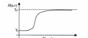
//High-Frequency-Emphasis Filters
Mat Butterworth_Homomorphic_Filter(Size sz, int D, int n, float high_h_v_TB, float low_h_v_TB,Mat& realIm)
{
    Mat single(sz.height, sz.width, CV_32F);
    cout <<sz.width <<" "<< sz.height<<endl;
    Point centre = Point(sz.height/, sz.width/);
    double radius;
    float upper = (high_h_v_TB * );
    float lower = (low_h_v_TB * );
    long dpow = D*D;
    float W = (upper - lower);

    for(int i = ; i < sz.height; i++)
    {
        for(int j = ; j < sz.width; j++)
        {
            radius = pow((float)(i - centre.x), ) + pow((float) (j - centre.y), );
            float r = exp(-n*radius/dpow);
            if(radius < )
                single.at<float>(i,j) = upper;
            else
                single.at<float>(i,j) =W*( - r) + lower;
        }
    }

    single.copyTo(realIm);
    Mat butterworth_complex;
    //make two channels to match complex
    Mat butterworth_channels[] = {Mat_<float>(single), Mat::zeros(sz, CV_32F)};
    merge(butterworth_channels, , butterworth_complex);

    return butterworth_complex;
}
DFT變換:
//DFT 傳回功率譜Power
Mat Fourier_Transform(Mat frame_bw, Mat& image_complex,Mat &image_phase, Mat &image_mag)
{
    Mat frame_log;
    frame_bw.convertTo(frame_log, CV_32F);
    frame_log = frame_log/;
    /*Take the natural log of the input (compute log( + Mag)*/
    frame_log += ;
    log( frame_log, frame_log); // log(1 + Mag)

    /* Expand the image to an optimal size
    The performance of the DFT depends of the image size. It tends to be the fastest for image sizes that are multiple of ,  or
    We can use the copyMakeBorder() function to expand the borders of an image.*/
    Mat padded;
    int M = getOptimalDFTSize(frame_log.rows);
    int N = getOptimalDFTSize(frame_log.cols);
    copyMakeBorder(frame_log, padded, , M - frame_log.rows, , N - frame_log.cols, BORDER_CONSTANT, Scalar::all());

    /*Make place for both the complex and real values
    The result of the DFT is a complex. Then the result is  images (Imaginary + Real), and the frequency domains range is much larger than the spatial one. Therefore we need to store in float !
    That's why we will convert our input image "padded" to float and expand it to another channel to hold the complex values.
    Planes is an arrow of  matrix (planes[] = Real part, planes[] = Imaginary part)*/
    Mat image_planes[] = {Mat_<float>(padded), Mat::zeros(padded.size(), CV_32F)};
    /*Creates one multichannel array out of several single-channel ones.*/
    merge(image_planes, , image_complex);

    /*Make the DFT
    The result of thee DFT is a complex image : "image_complex"*/
    dft(image_complex, image_complex);

    /***************************/
    //Create spectrum magnitude//
    /***************************/
    /*Transform the real and complex values to magnitude
    NB: We separe Real part to Imaginary part*/
    split(image_complex, image_planes);
    //Starting with this part we have the real part of the image in planes[0] and the imaginary in planes[1]
    phase(image_planes[], image_planes[], image_phase);
    magnitude(image_planes[], image_planes[], image_mag);

    //Power
    pow(image_planes[],,image_planes[]);
    pow(image_planes[],,image_planes[]);

    Mat Power = image_planes[] + image_planes[];

    return Power;
}
IDFT變換
void Inv_Fourier_Transform(Mat input, Mat& inverseTransform)
{
    /*Make the IDFT*/
    Mat result;
    idft(input, result,DFT_SCALE);
    /*Take the exponential*/
    exp(result, result);

    vector<Mat> planes;
    split(result,planes);
    magnitude(planes[],planes[],planes[]);
    planes[] = planes[] - ;
    normalize(planes[],planes[],,,CV_MINMAX);

    planes[].convertTo(inverseTransform,CV_8U);
}
頻譜移位
//SHIFT
void Shifting_DFT(Mat &fImage)
{
    //For visualization purposes we may also rearrange the quadrants of the result, so that the origin (0,0), corresponds to the image center.
    Mat tmp, q0, q1, q2, q3;

    /*First crop the image, if it has an odd number of rows or columns.
    Operator & bit to bit by - (two's complement : - = ..) to eliminate the first bit ^ (In case of odd number on row or col, we take the even number in below)*/
    fImage = fImage(Rect(, , fImage.cols & -, fImage.rows & -));
    int cx = fImage.cols/;
    int cy = fImage.rows/;

    /*Rearrange the quadrants of Fourier image so that the origin is at the image center*/
    q0 = fImage(Rect(, , cx, cy));
    q1 = fImage(Rect(cx, , cx, cy));
    q2 = fImage(Rect(, cy, cx, cy));
    q3 = fImage(Rect(cx, cy, cx, cy));

    /*We reverse each quadrant of the frame with its other quadrant diagonally opposite*/
    /*We reverse q0 and q3*/
    q0.copyTo(tmp);
    q3.copyTo(q0);
    tmp.copyTo(q3);

    /*We reverse q1 and q2*/
    q1.copyTo(tmp);
    q2.copyTo(q1);
    tmp.copyTo(q2);
}
主函數:
void homomorphicFiltering(Mat src,Mat& dst)
{
    Mat img;
    Mat imgHls;
    vector<Mat> vHls;

    if(src.channels() == )
    {
        cvtColor(src,imgHls,CV_BGR2HSV);
        split(imgHls,vHls);
        vHls[].copyTo(img);
    }
    else
        src.copyTo(img);

    //DFT
    //cout<<"DFT "<<endl;
    Mat img_complex,img_mag,img_phase;
    Mat fpower = Fourier_Transform(img,img_complex,img_phase,img_mag);
    Shifting_DFT(img_complex);
    Shifting_DFT(fpower);
    //int D0 = getRadius(fpower,0.15);
    int D0 = ;
    int n = ;
    int w = img_complex.cols;
    int h = img_complex.rows;
    //BHPF
//  Mat filter,filter_complex;
//  filter = BHPF(h,w,D0,n);
//  Mat planes[] = {Mat_<float>(filter), Mat::zeros(filter.size(), CV_32F)};
//  merge(planes,2,filter_complex);

    int rH = ;
    int rL = ;
    Mat filter,filter_complex;
    filter_complex = Butterworth_Homomorphic_Filter(Size(w,h),D0,n,rH,rL,filter);

    //do mulSpectrums on the full dft
    mulSpectrums(img_complex, filter_complex, filter_complex, );

    Shifting_DFT(filter_complex);
    //IDFT
    Mat result;
    Inv_Fourier_Transform(filter_complex,result);

    if(src.channels() == )
    {
        vHls.at()= result(Rect(,,src.cols,src.rows));
        merge(vHls,imgHls);
        cvtColor(imgHls, dst, CV_HSV2BGR);
    }
    else
        result.copyTo(dst);

}